Plotting sparr objects
Source:R/plot.bivden.R, R/plot.msden.R, R/plot.rrs.R, and 2 more
plotsparr.Rd# S3 method for bivden
plot(
x,
what = c("z", "edge", "bw"),
add.pts = FALSE,
auto.axes = TRUE,
override.par = TRUE,
...
)
# S3 method for msden
plot(x, what = c("z", "edge", "bw"), sleep = 0.2, override.par = TRUE, ...)
# S3 method for rrs
plot(
x,
auto.axes = TRUE,
tol.show = TRUE,
tol.type = c("upper", "lower", "two.sided"),
tol.args = list(levels = 0.05, lty = 1, drawlabels = TRUE),
...
)
# S3 method for rrst
plot(
x,
tselect = NULL,
type = c("joint", "conditional"),
fix.range = FALSE,
tol.show = TRUE,
tol.type = c("upper", "lower", "two.sided"),
tol.args = list(levels = 0.05, lty = 1, drawlabels = TRUE),
sleep = 0.2,
override.par = TRUE,
expscale = FALSE,
...
)
# S3 method for stden
plot(
x,
tselect = NULL,
type = c("joint", "conditional"),
fix.range = FALSE,
sleep = 0.2,
override.par = TRUE,
...
)Arguments
- x
- what
A character string to select plotting of result (
"z"; default); edge-correction surface ("edge"); or variable bandwidth surface ("bw").- add.pts
Logical value indicating whether to add the observations to the image plot using default
points.- auto.axes
Logical value indicating whether to display the plot with automatically added x-y axes and an `L' box in default styles.
- override.par
Logical value indicating whether to override the existing graphics device parameters prior to plotting, resetting
mfrowandmar. See `Details' for when you might want to disable this.- ...
Additional graphical parameters to be passed to
plot.im, or in one instance, toplot.ppp(see `Details').- sleep
Single positive numeric value giving the amount of time (in seconds) to
Sys.sleepbefore drawing the next image in the animation.- tol.show
Logical value indicating whether to show pre-computed tolerance contours on the plot(s). The object
xmust already have the relevant p-value surface(s) stored in order for this argument to have any effect.- tol.type
A character string used to control the type of tolerance contour displayed; a test for elevated risk (
"upper"), decreased risk ("lower"), or a two-tailed test (two.sided).- tol.args
A named list of valid arguments to be passed directly to
contourto control the appearance of plotted contours. Commonly used items arelevels,lty,lwdanddrawlabels.- tselect
Either a single numeric value giving the time at which to return the plot, or a vector of length 2 giving an interval of times over which to plot. This argument must respect the stored temporal bound in
x$tlim, else an error will be thrown. By default, the full set of images (i.e. over the entire available time span) is plotted.- type
A character string to select plotting of joint/unconditional spatiotemporal estimate (default) or conditional spatial density given time.
- fix.range
Logical value indicating whether use the same color scale limits for each plot in the sequence. Ignored if the user supplies a pre-defined
colourmapto thecolargument, which is matched to...above and passed toplot.im. See `Examples'.- expscale
Logical value indicating whether to force a raw-risk scale. Useful for users wishing to plot a log-relative risk surface, but to have the raw-risk displayed on the colour ribbon.
Value
Plots to the relevant graphics device.
Details
In all instances, visualisation is deferred to
plot.im, for which there are a variety of
customisations available the user can access via .... The one
exception is when plotting observation-specific "diggle" edge
correction factors---in this instance, a plot of the spatial observations is
returned with size proportional to the influence of each correction weight.
When plotting a rrs object, a pre-computed p-value
surface (see argument tolerate in risk) will
automatically be superimposed at a significance level of 0.05. Greater
flexibility in visualisation is gained by using tolerance in
conjunction with contour.
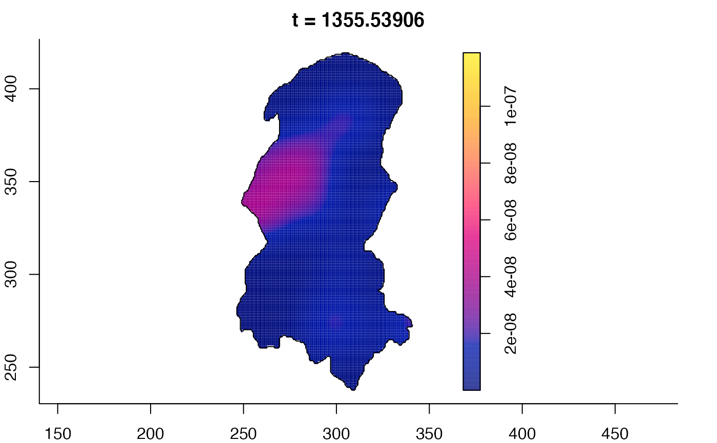
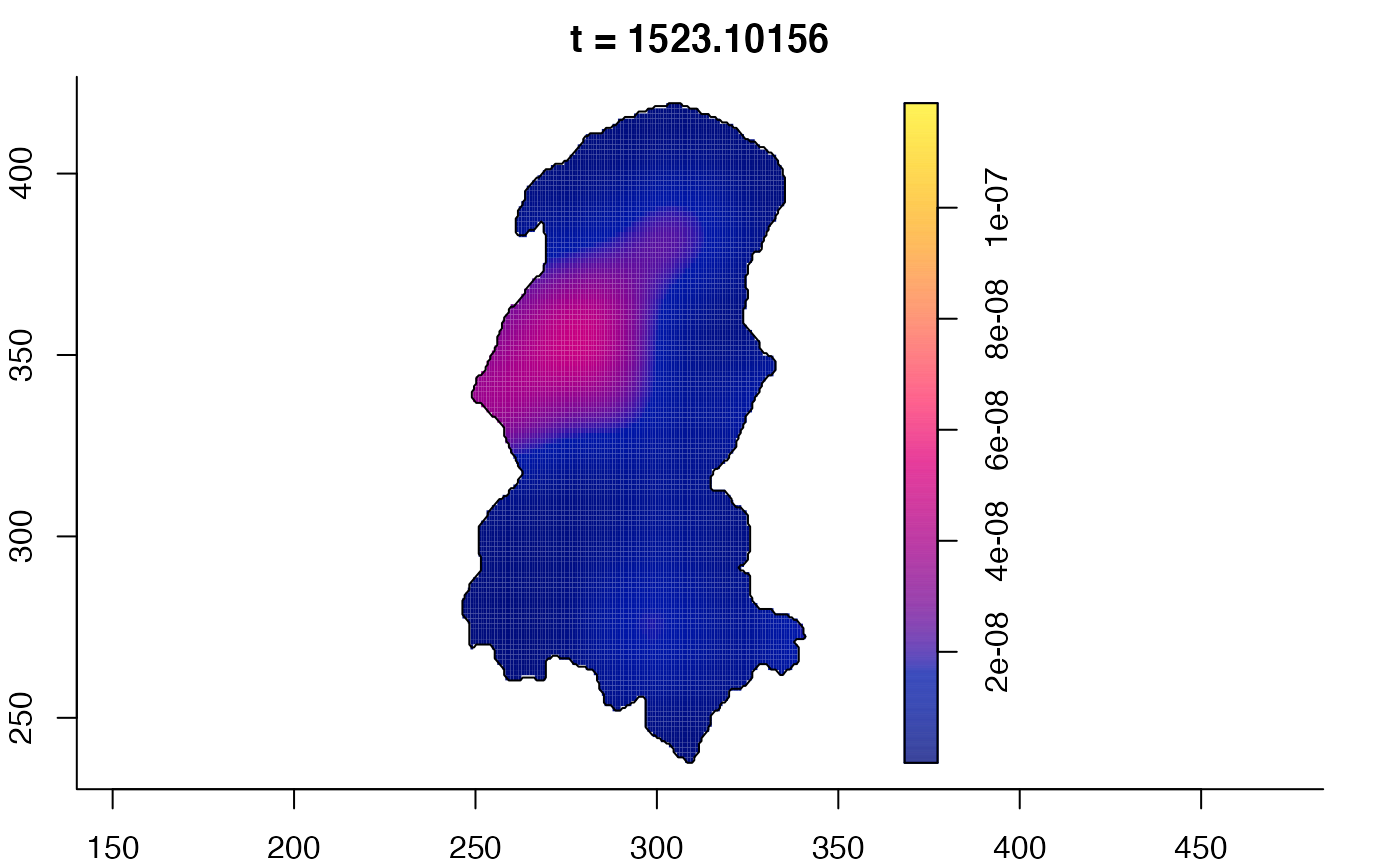
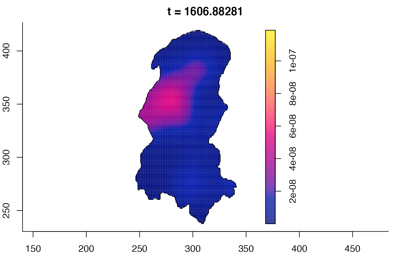
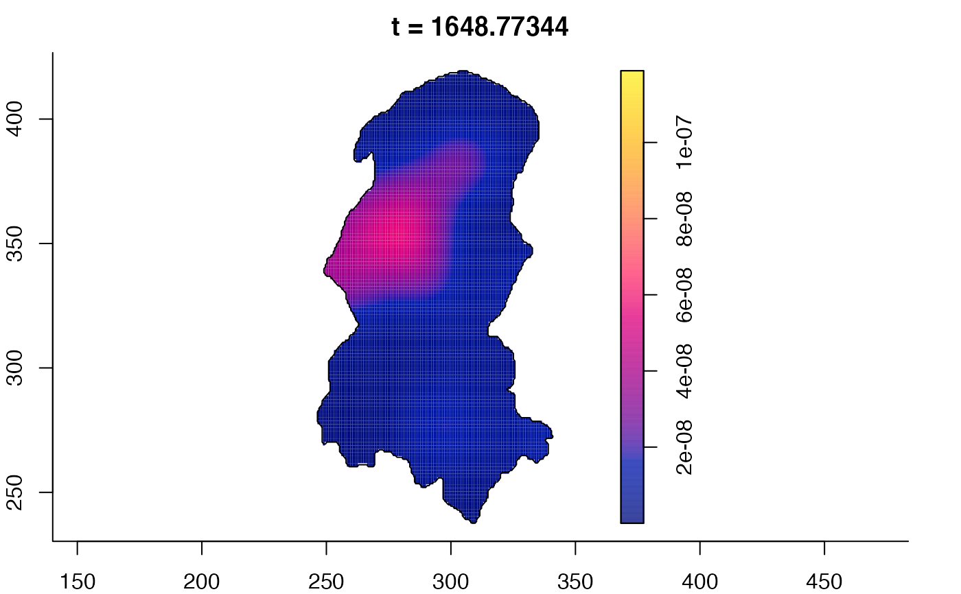
An msden, stden, or rrst object is plotted as an animation, one pixel image
after another, separated by sleep seconds. If instead you intend the
individual images to be plotted in an array of images, you should first set
up your plot device layout, and ensure override.par = FALSE so that
the function does not reset these device parameters itself. In such an
instance, one might also want to set sleep = 0.
Examples
# \donttest{
data(pbc)
data(fmd)
data(burk)
# 'bivden' object
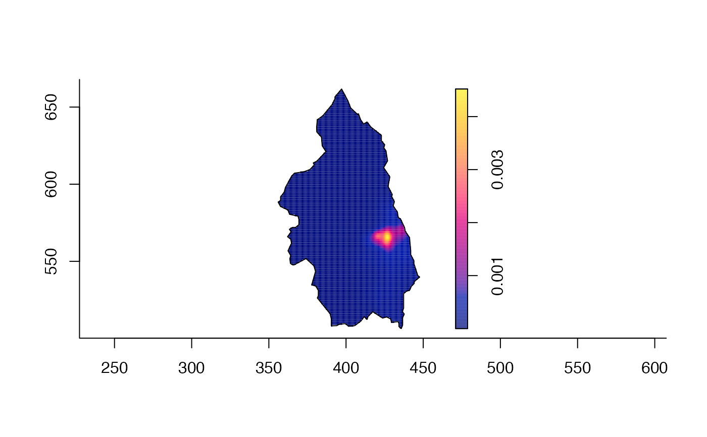
pbcden <- bivariate.density(split(pbc)$case,h0=3,hp=2,adapt=TRUE,davies.baddeley=0.05,verbose=FALSE)
plot(pbcden)
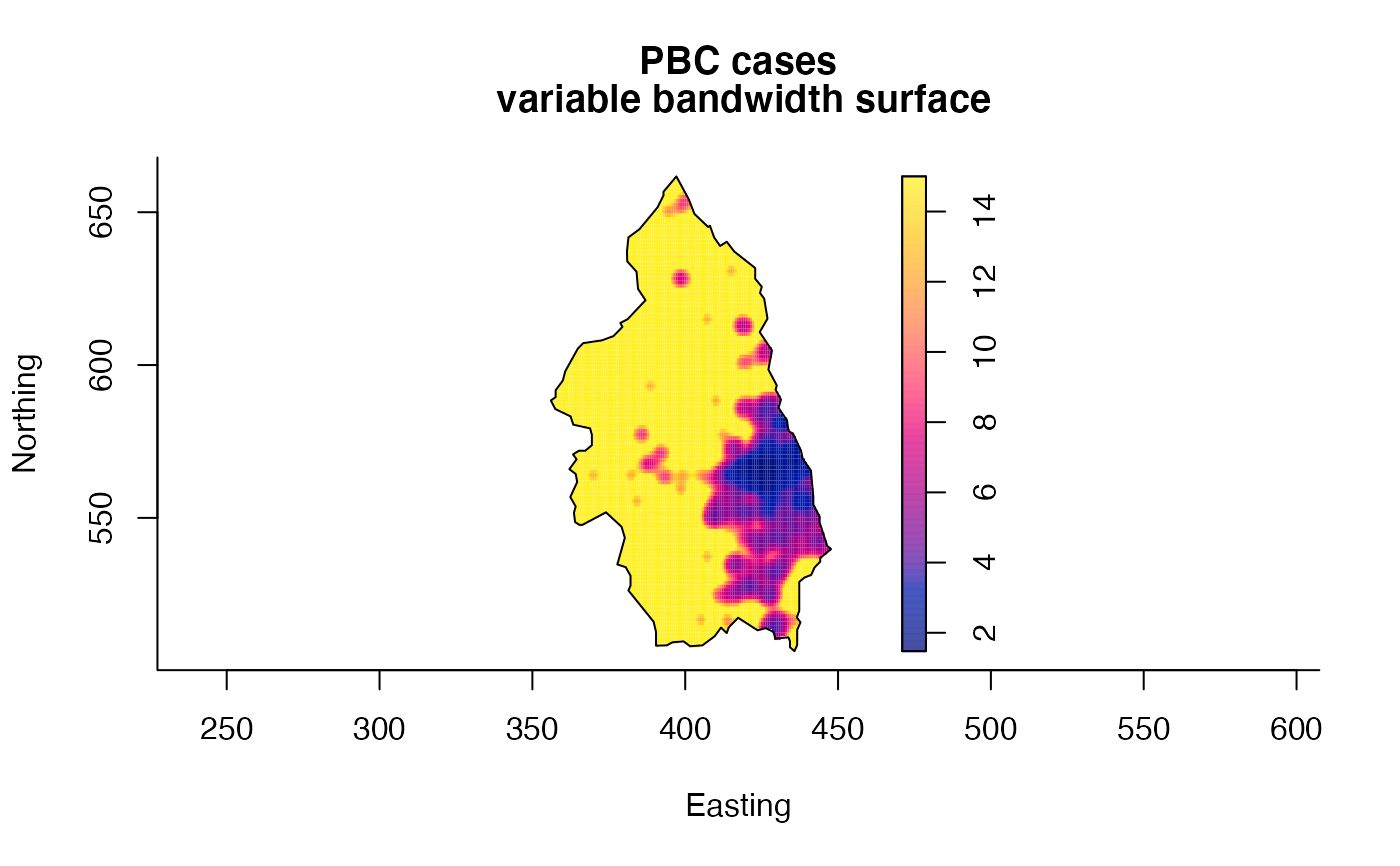
 plot(pbcden,what="bw",main="PBC cases\n variable bandwidth surface",xlab="Easting",ylab="Northing")
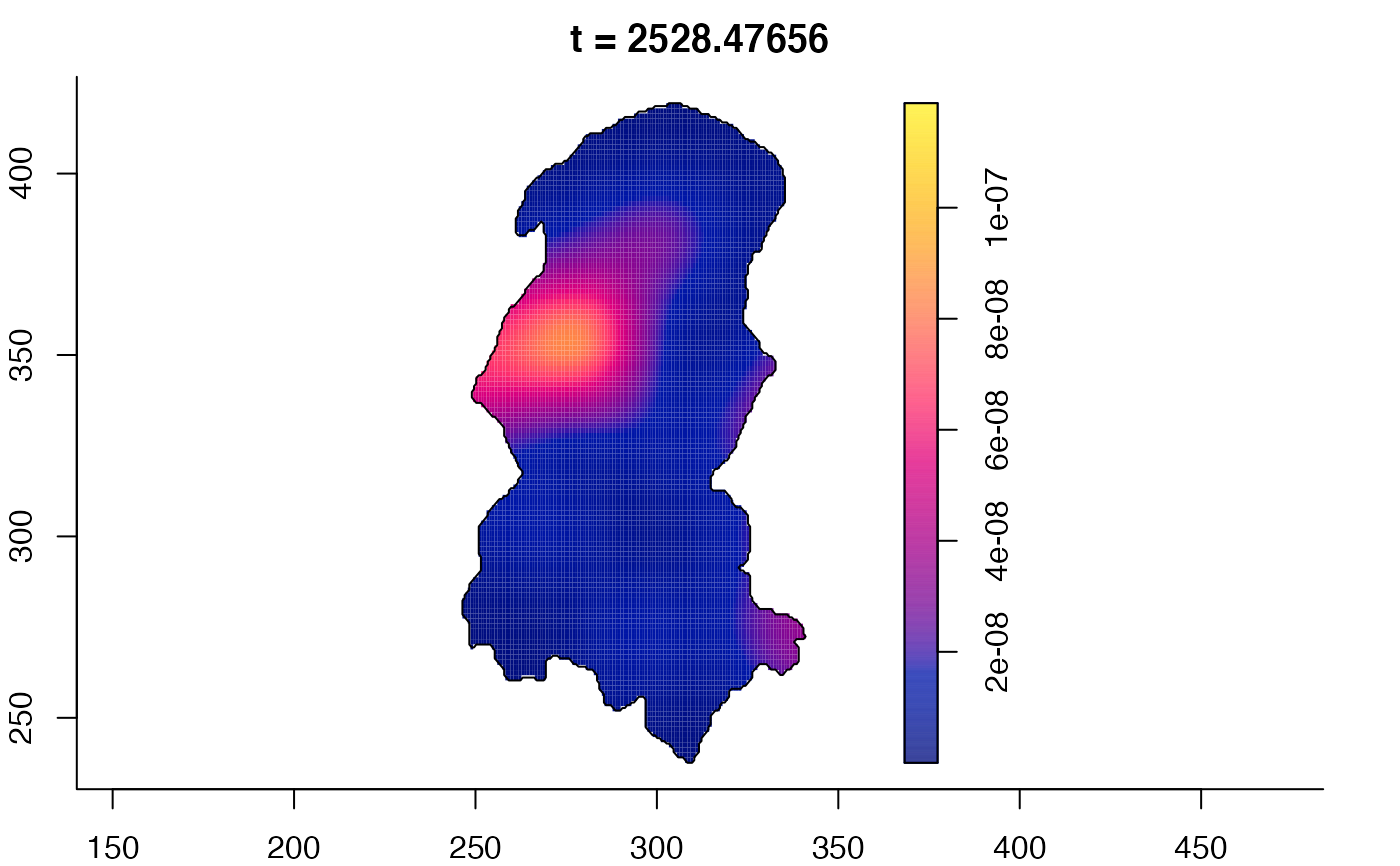
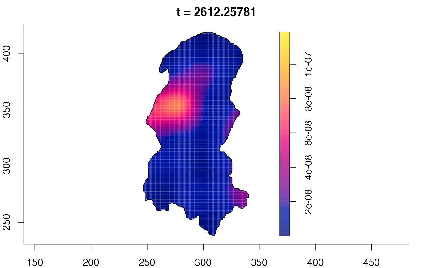
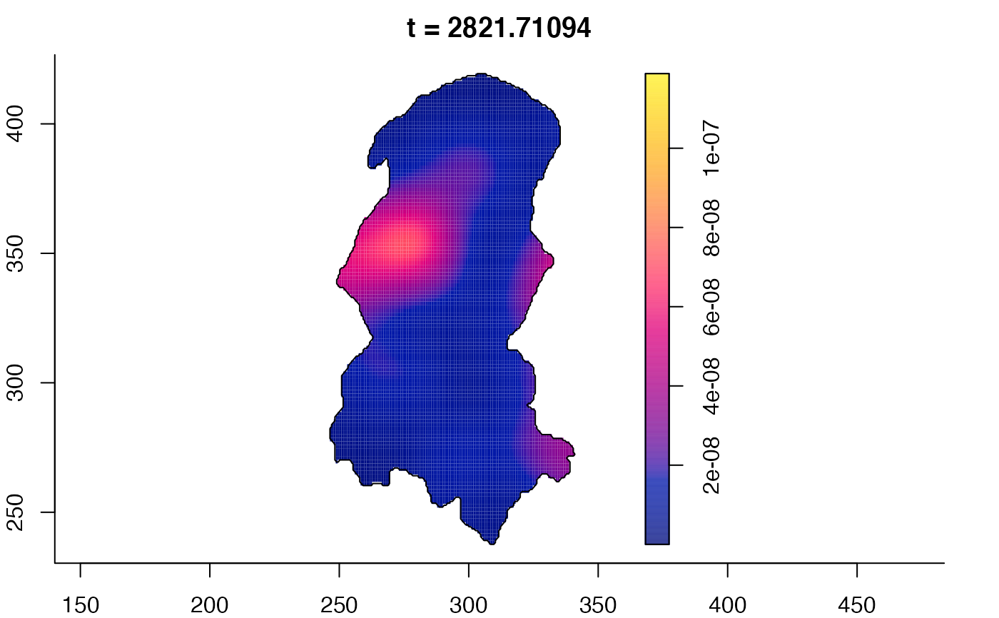
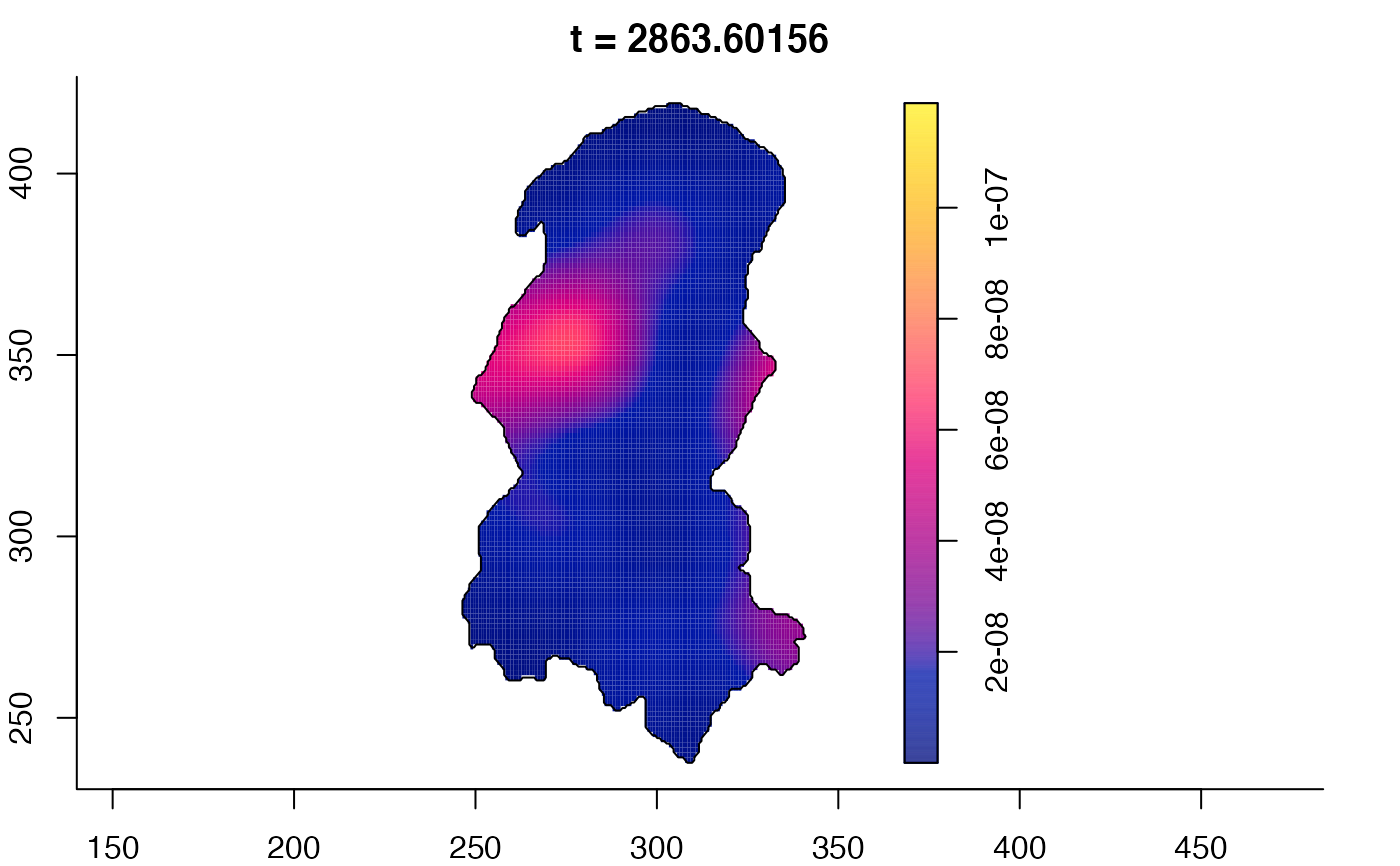
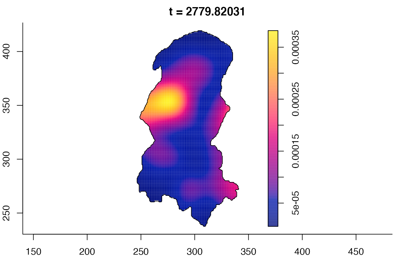
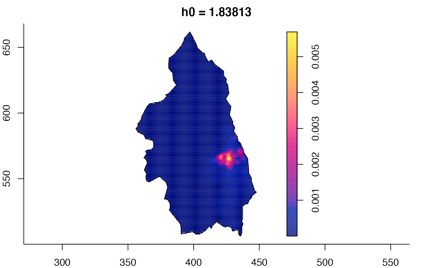
 # 'stden' object
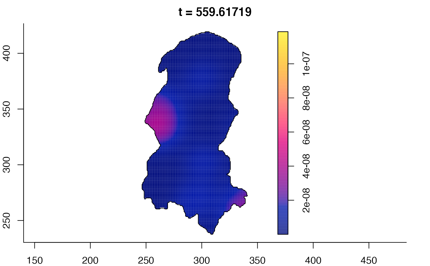
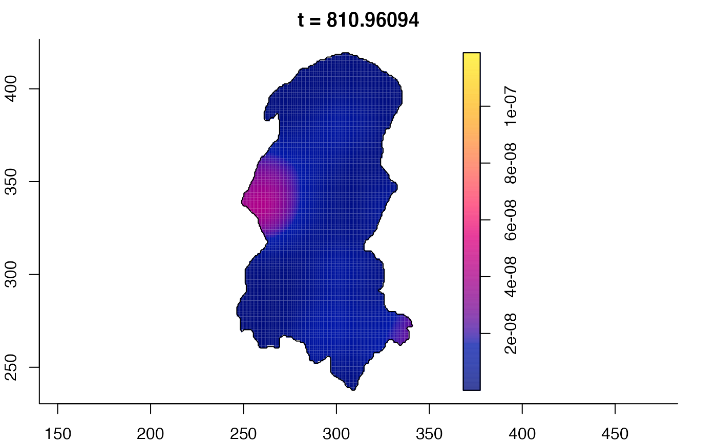
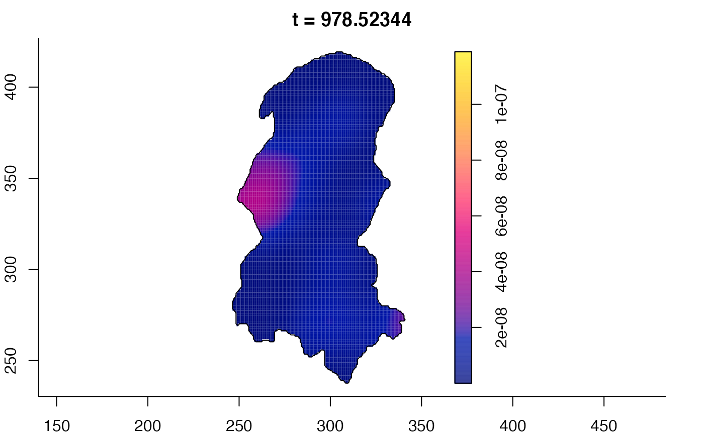
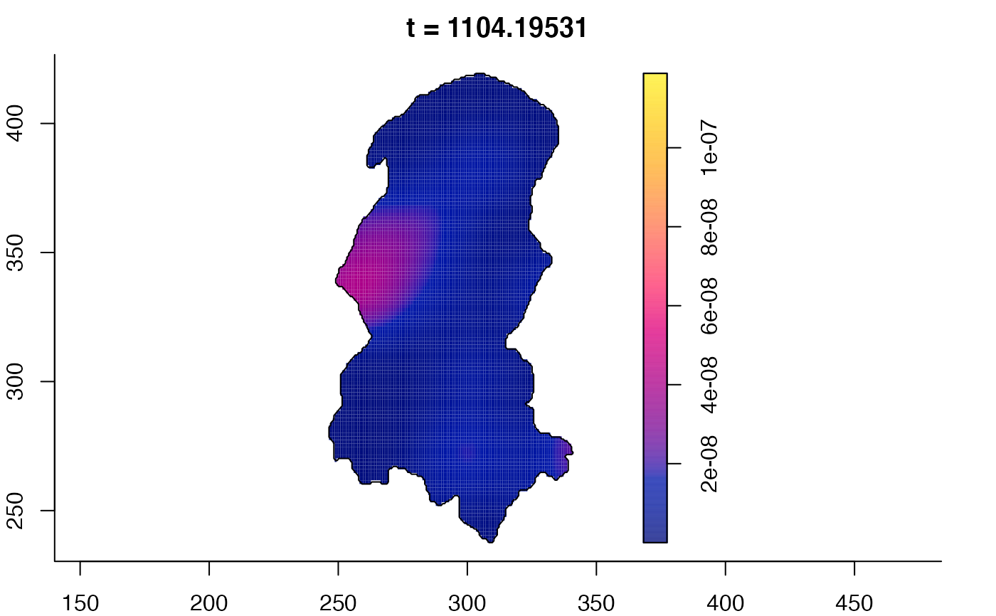
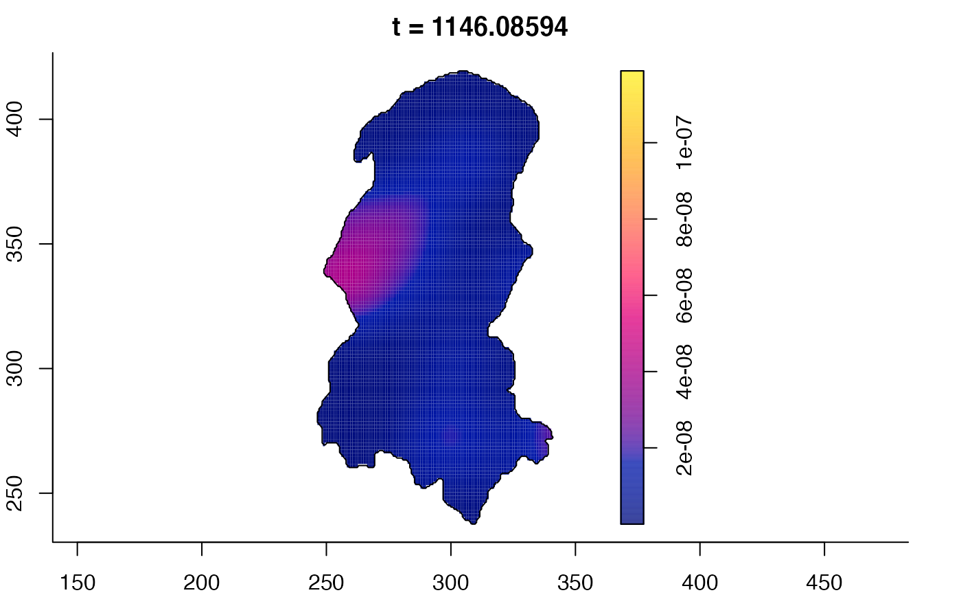
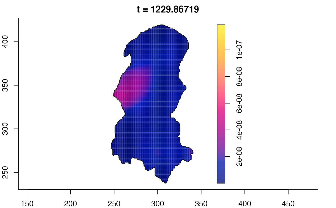
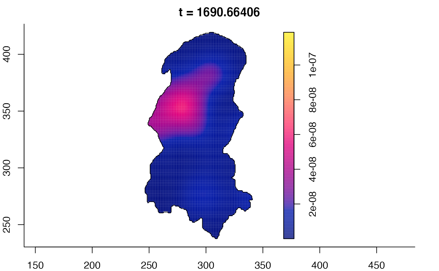
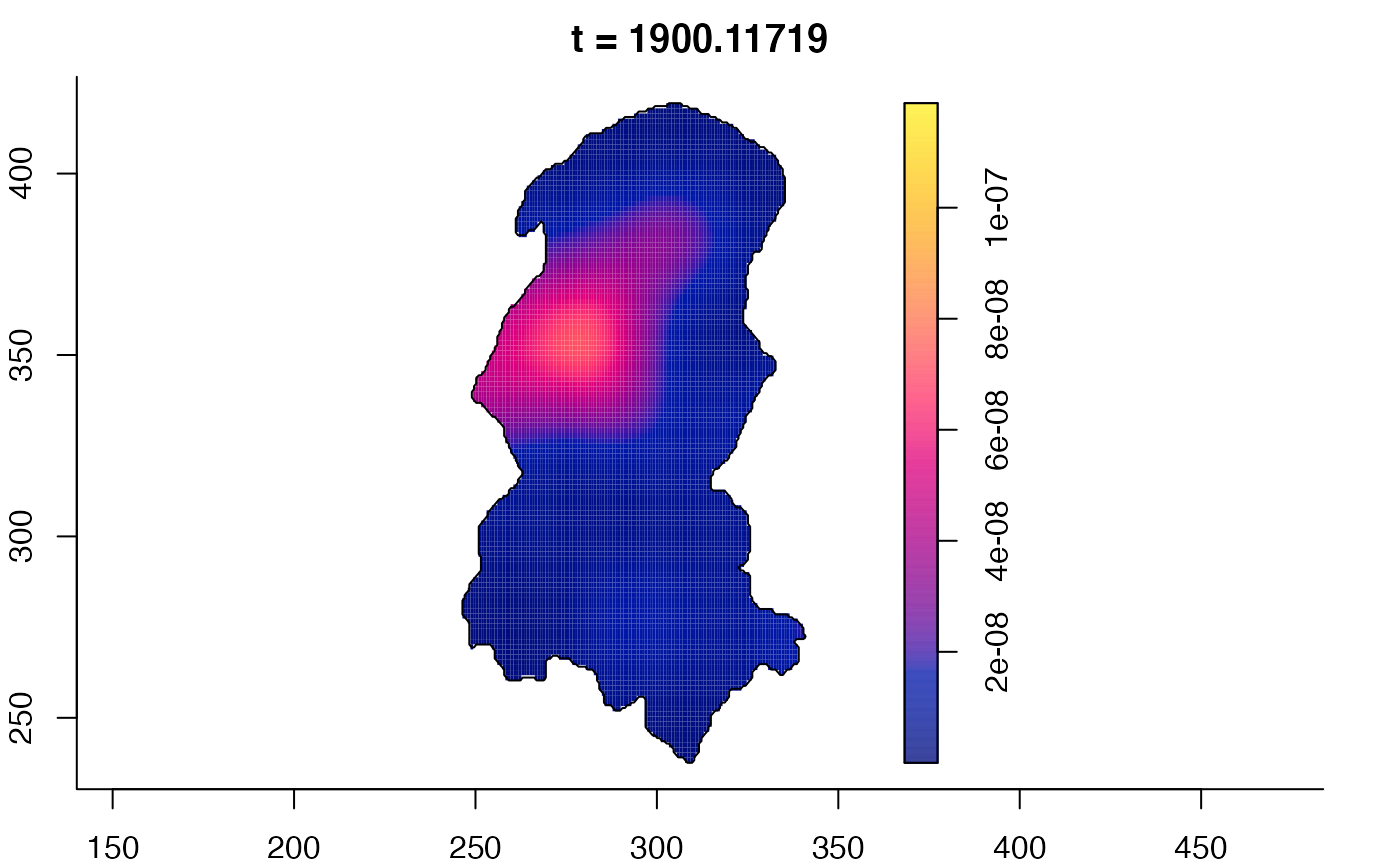
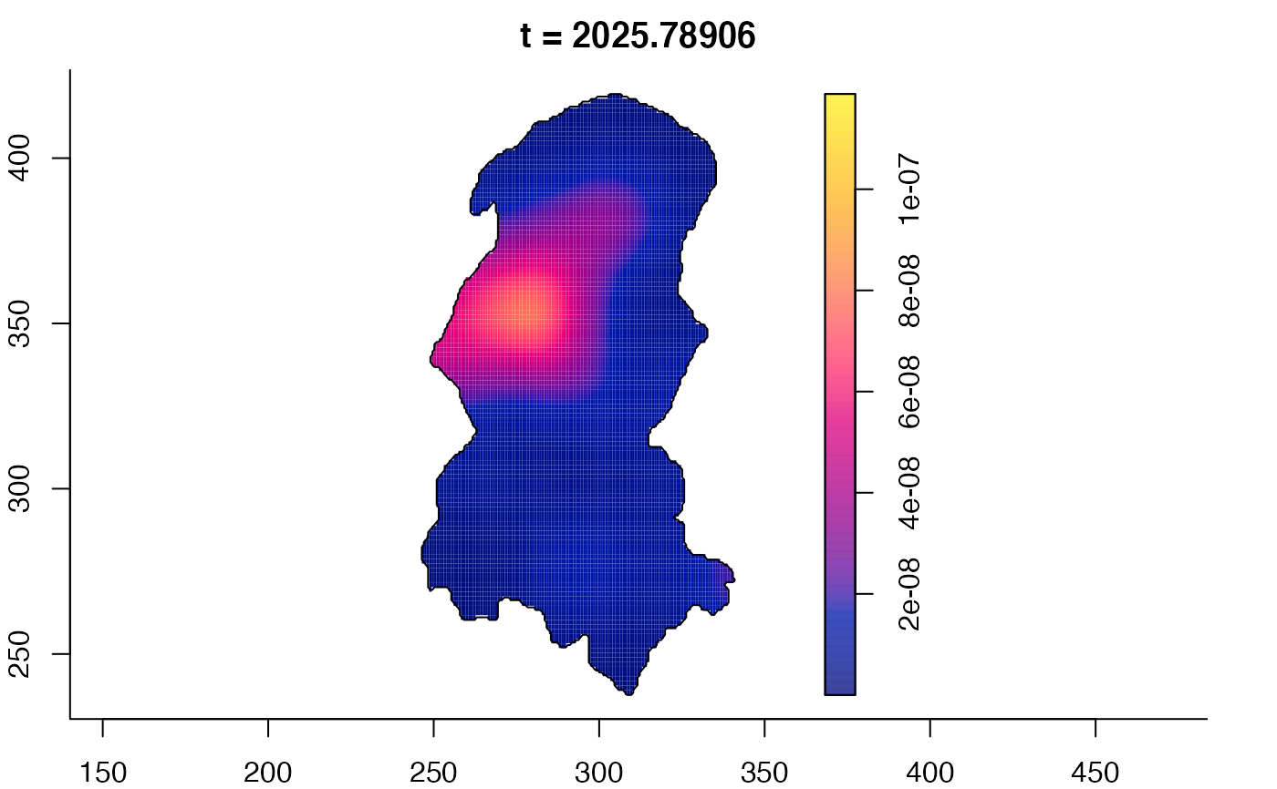
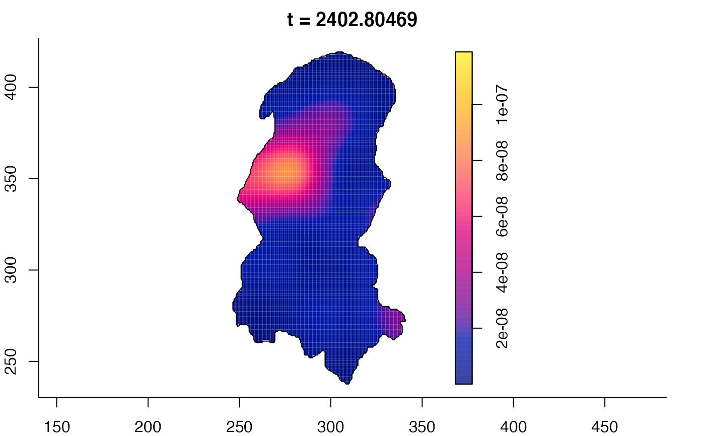
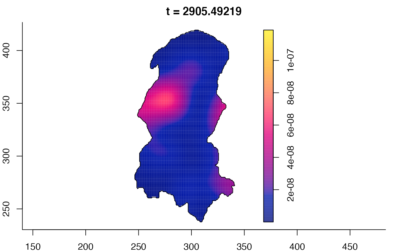
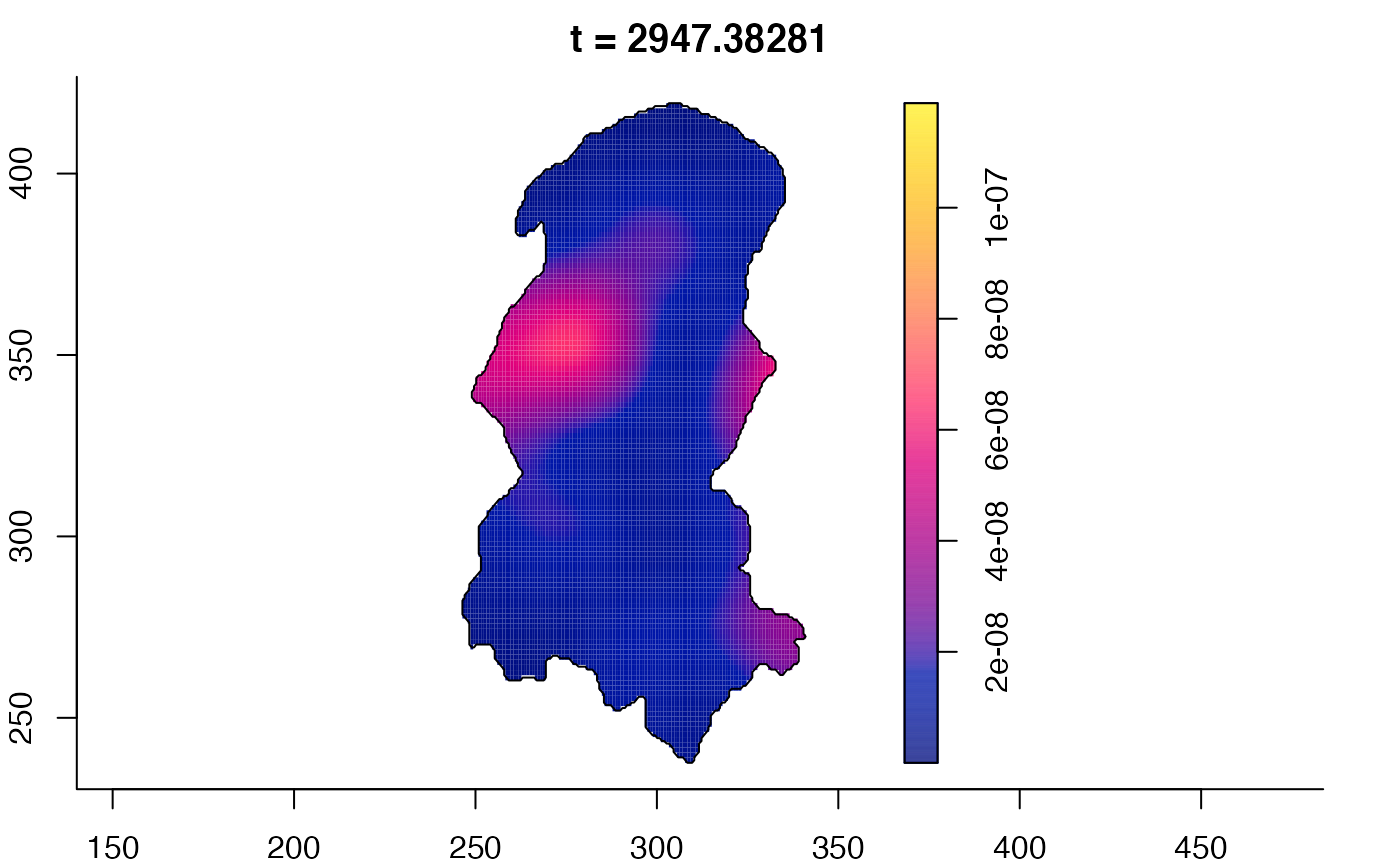
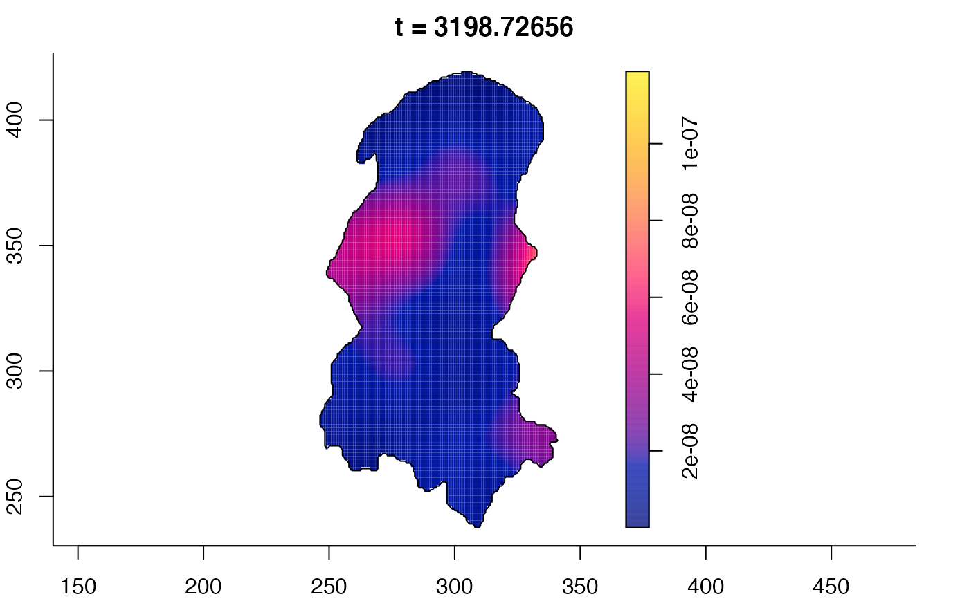
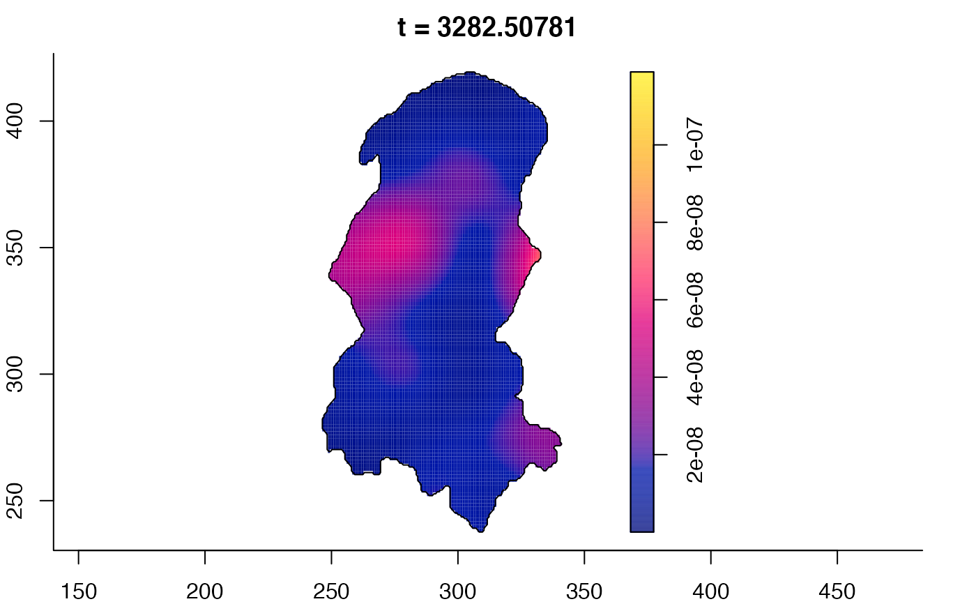
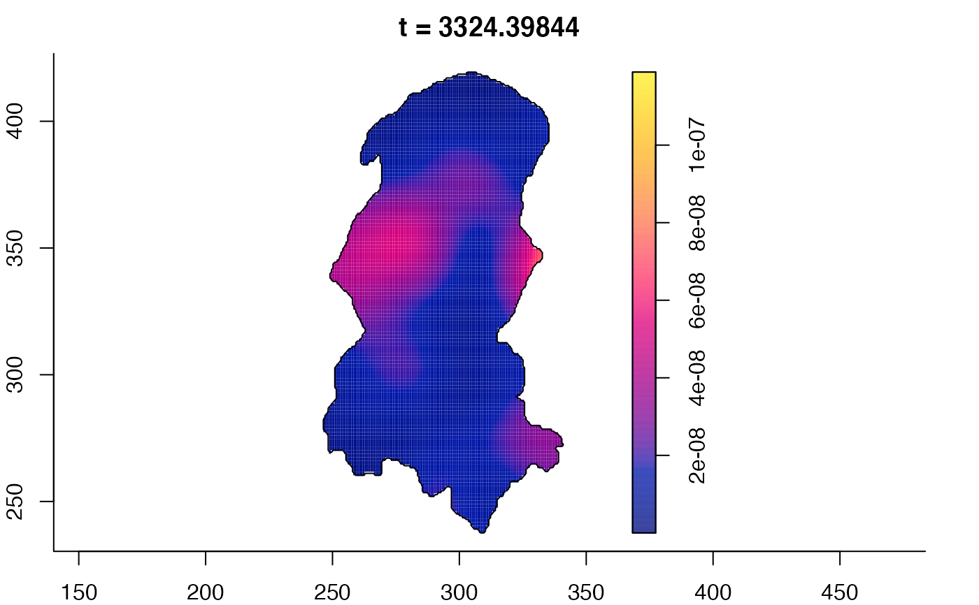
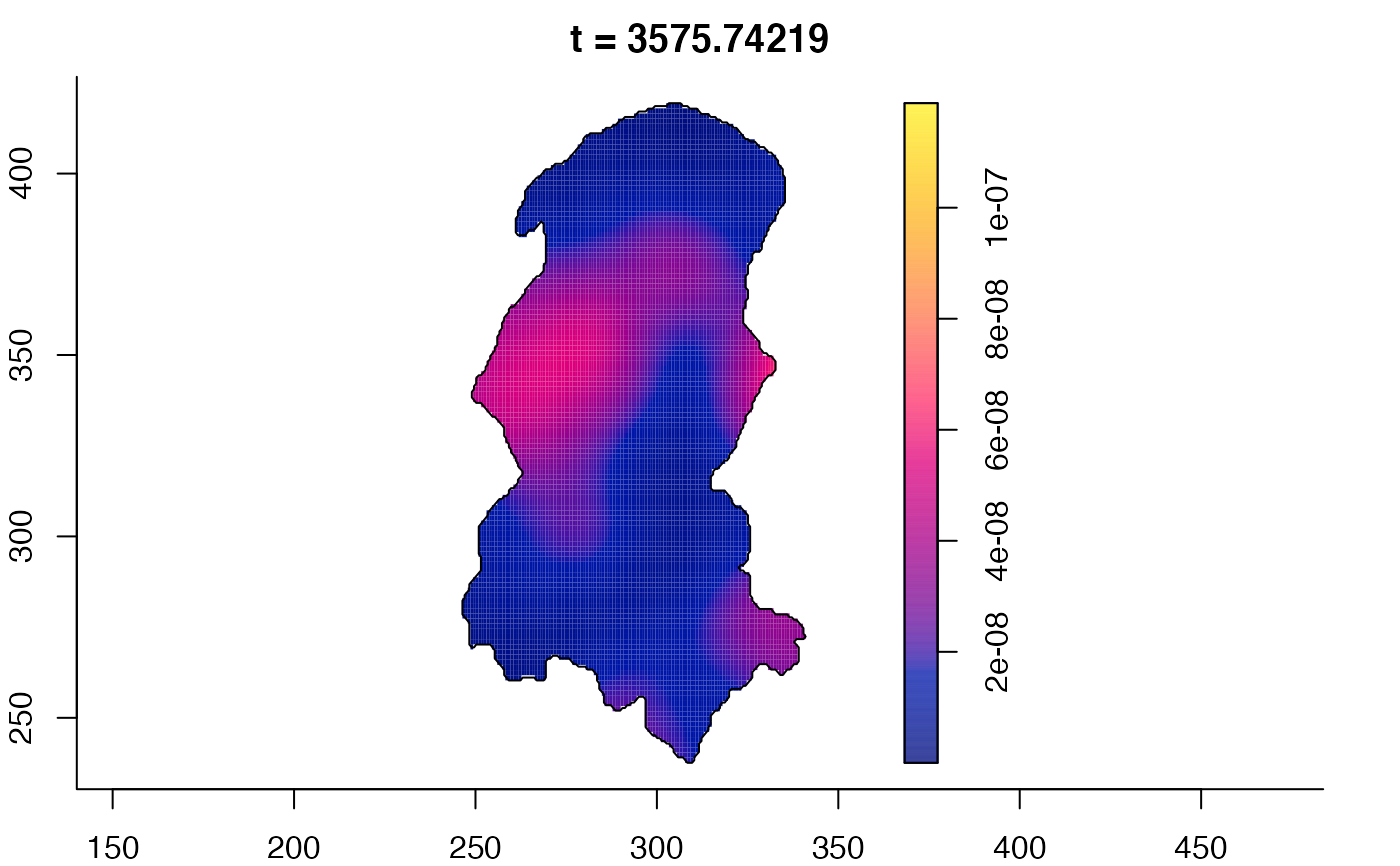
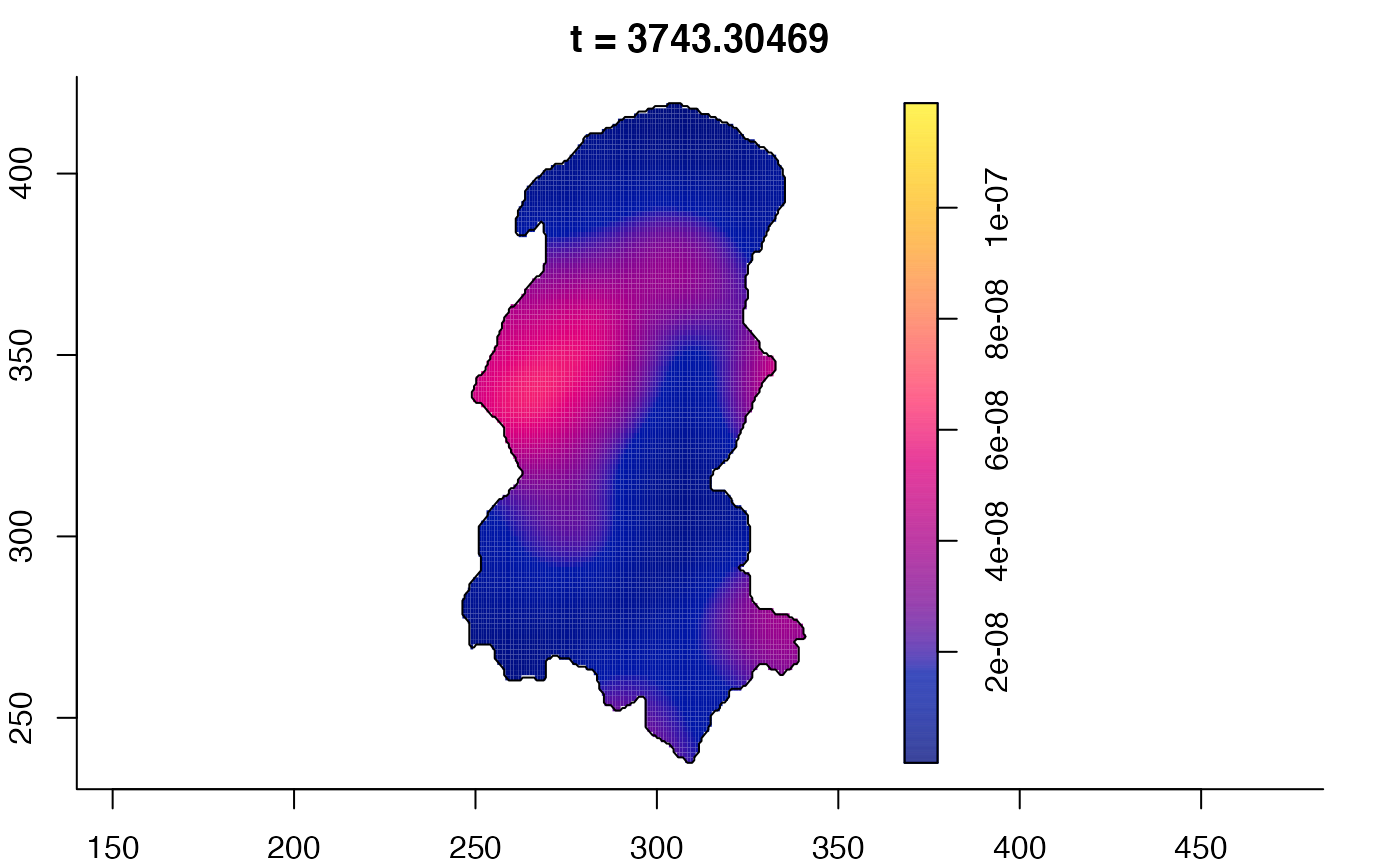
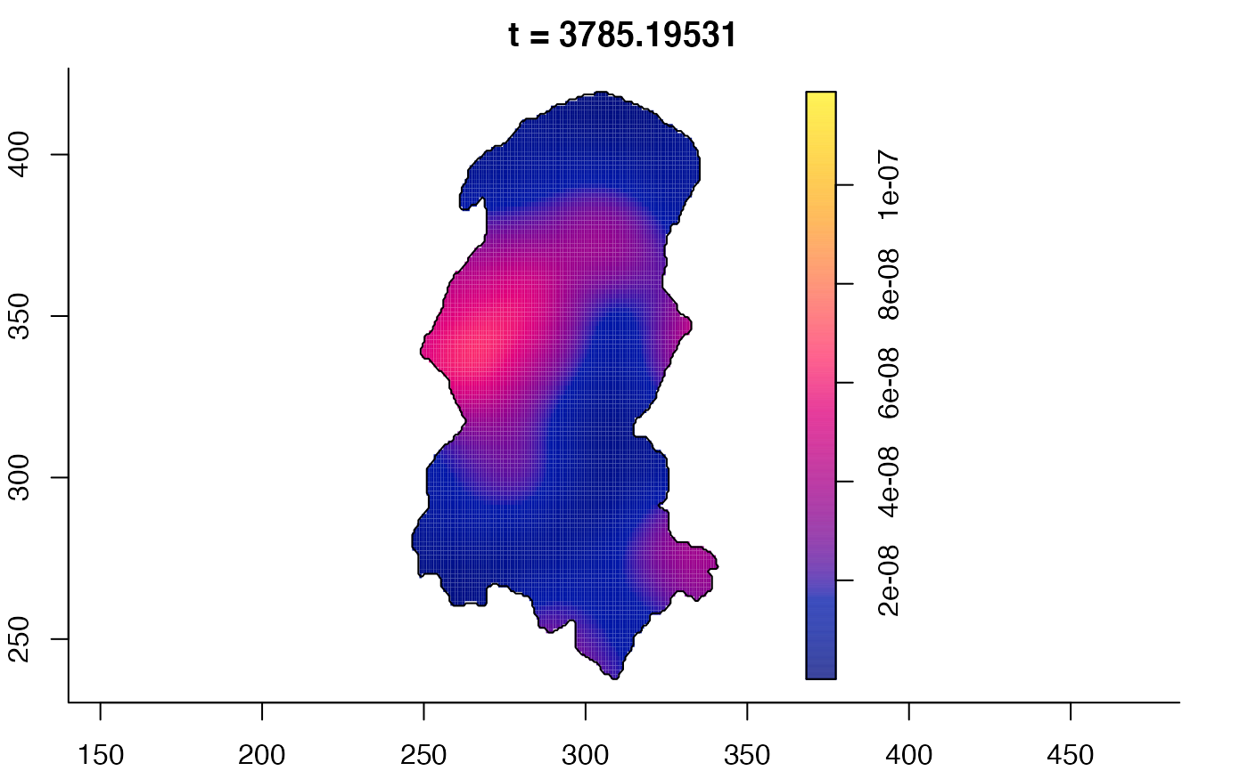
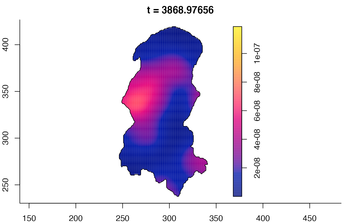
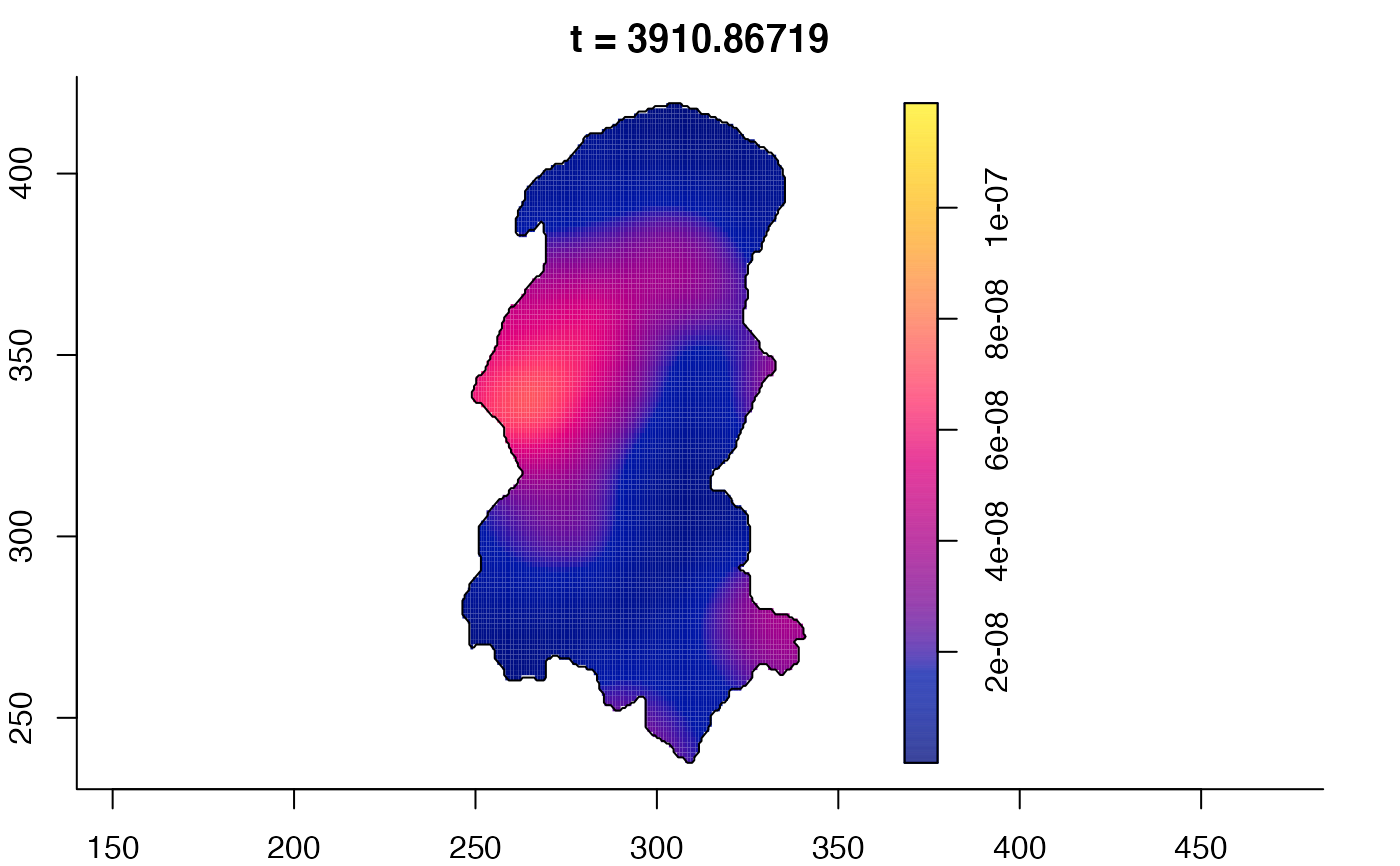
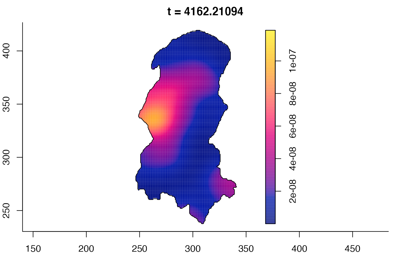
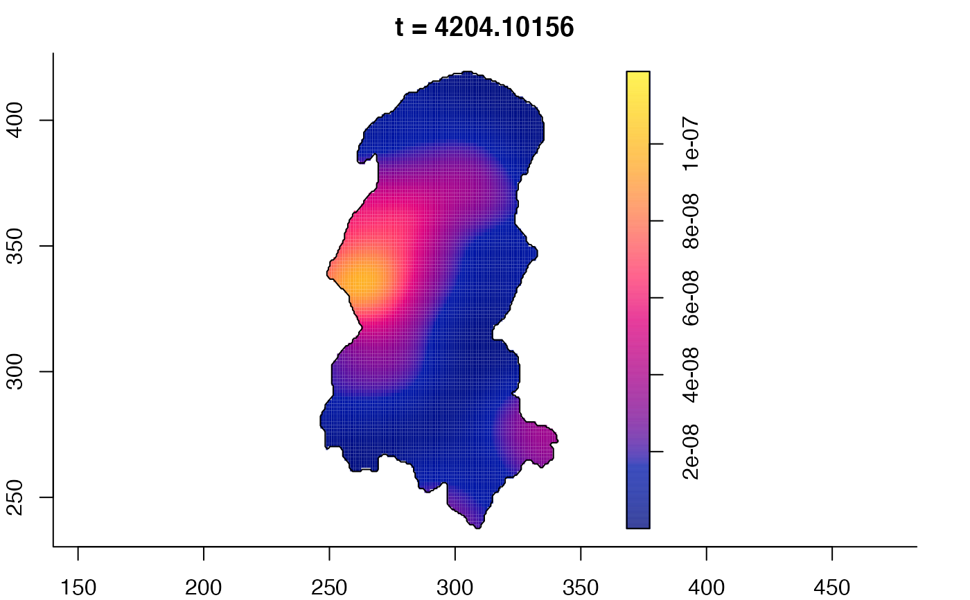
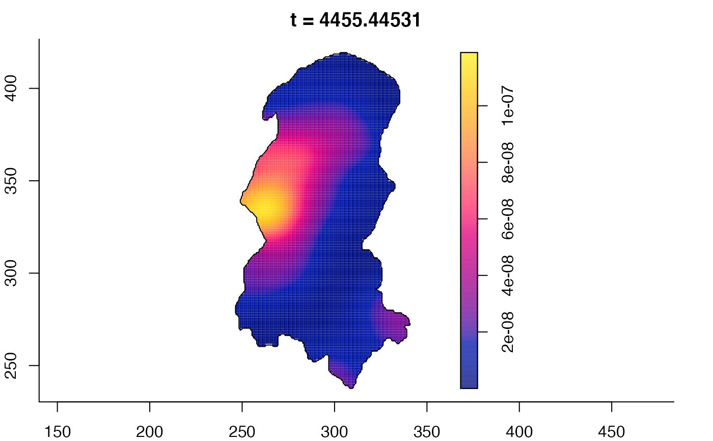
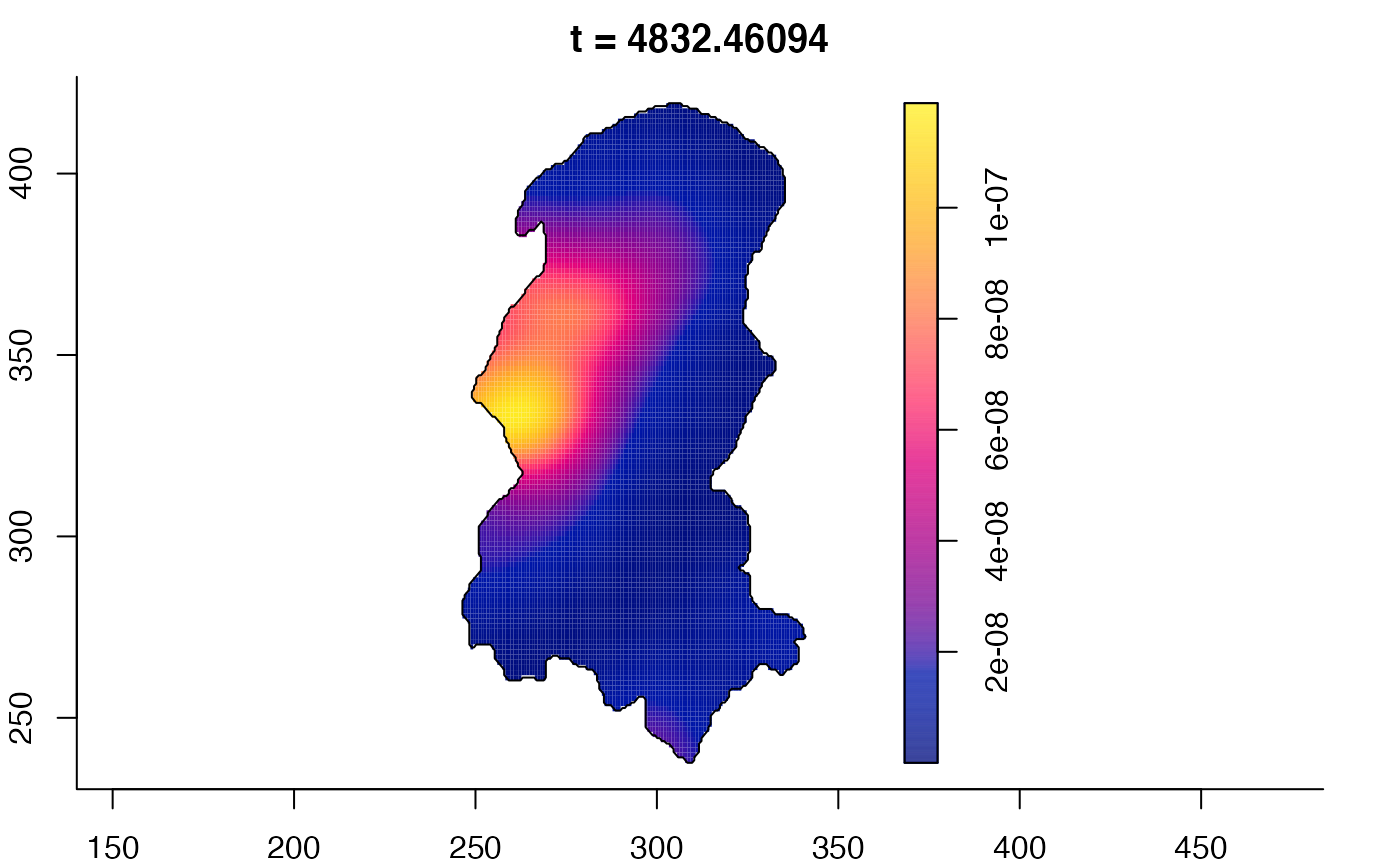
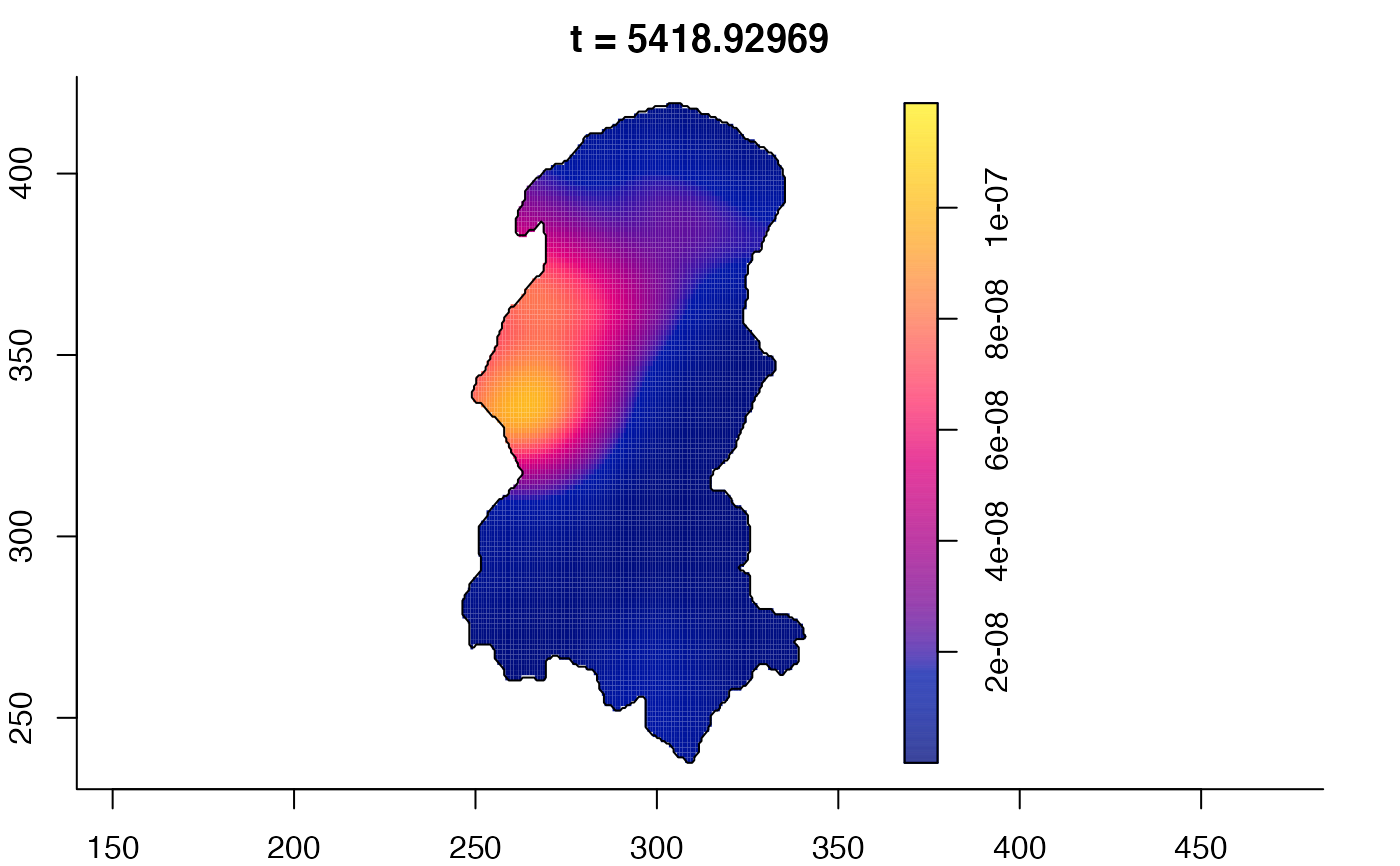
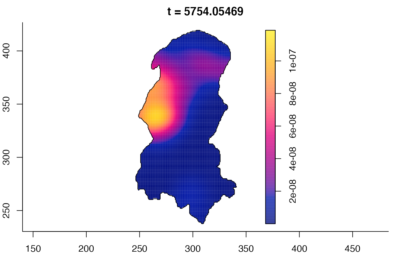
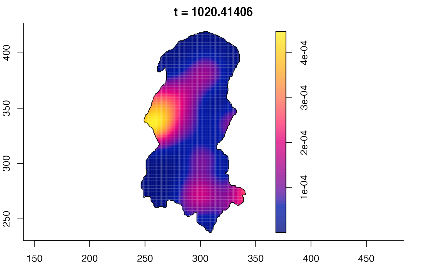
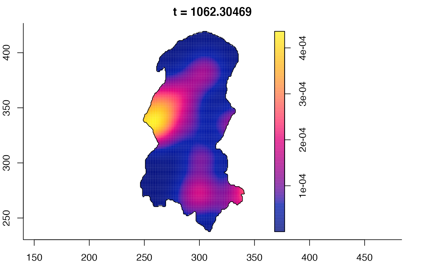
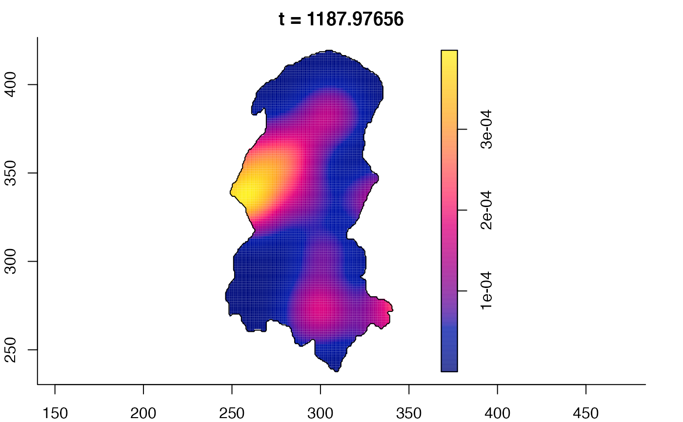
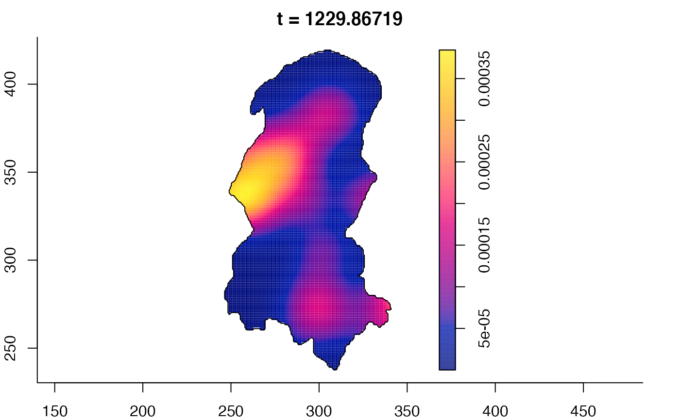
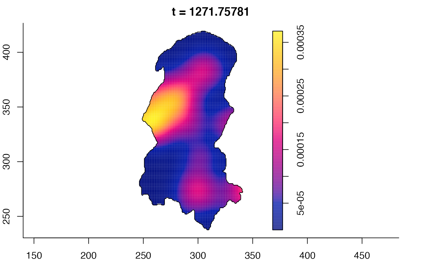
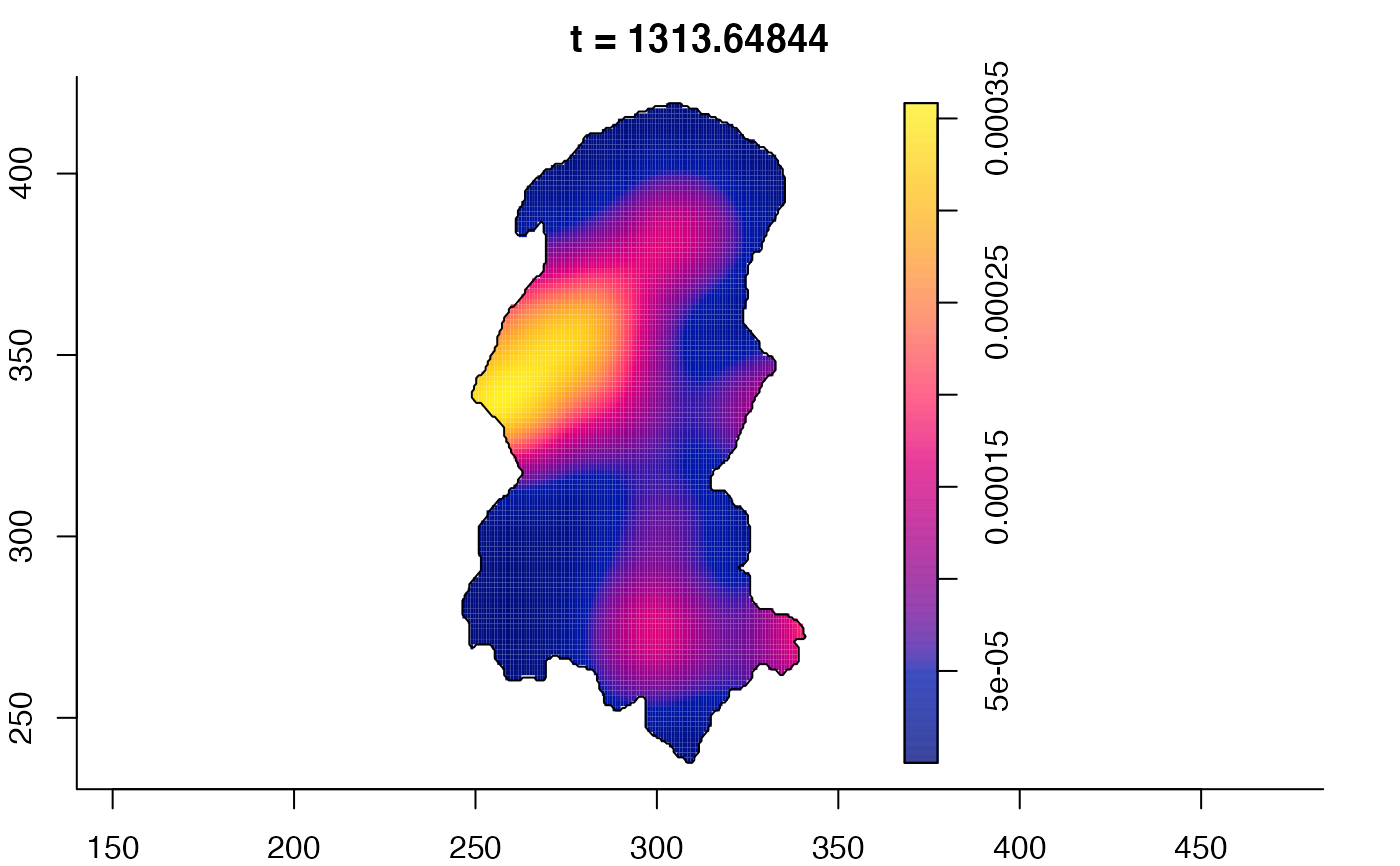
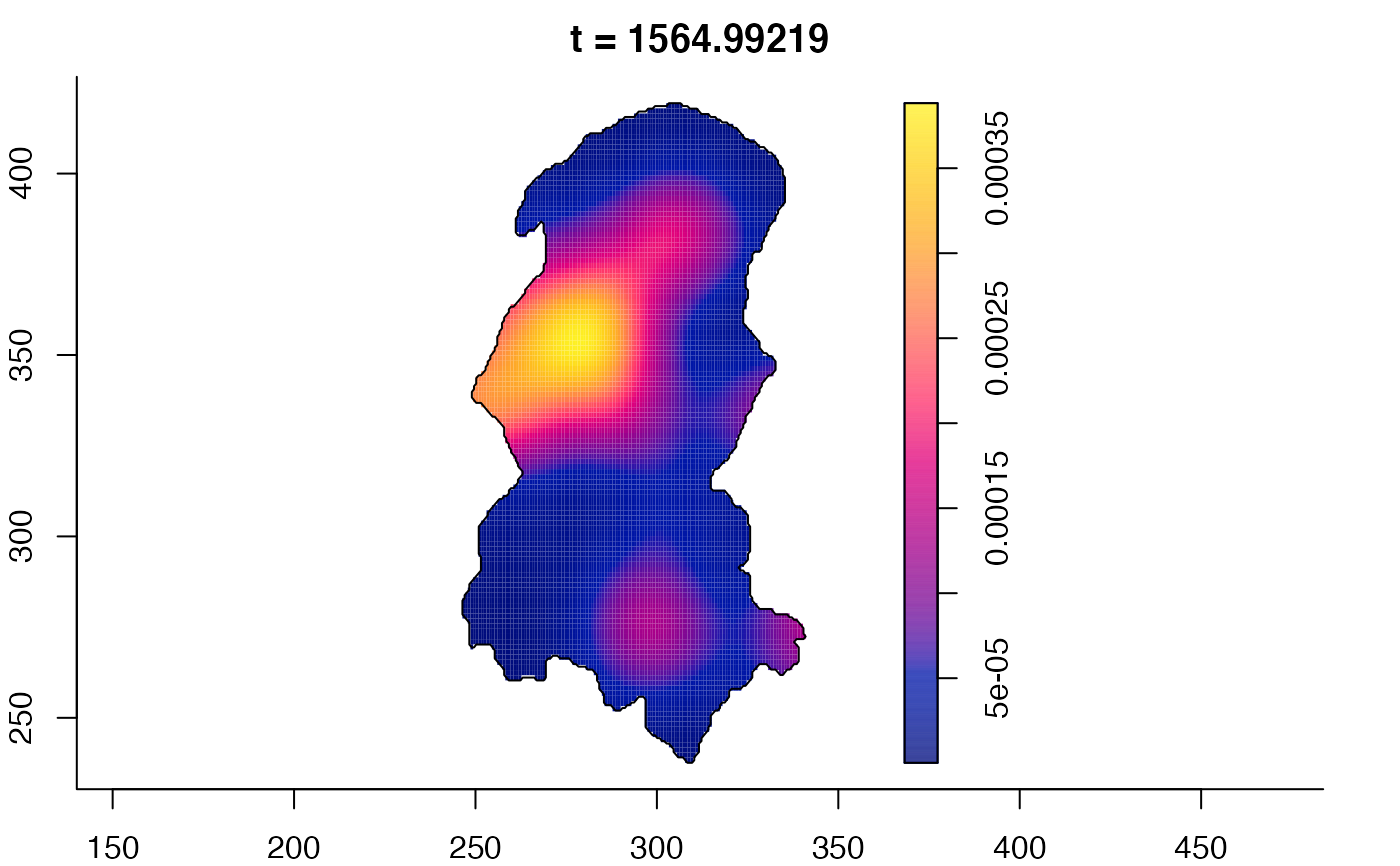
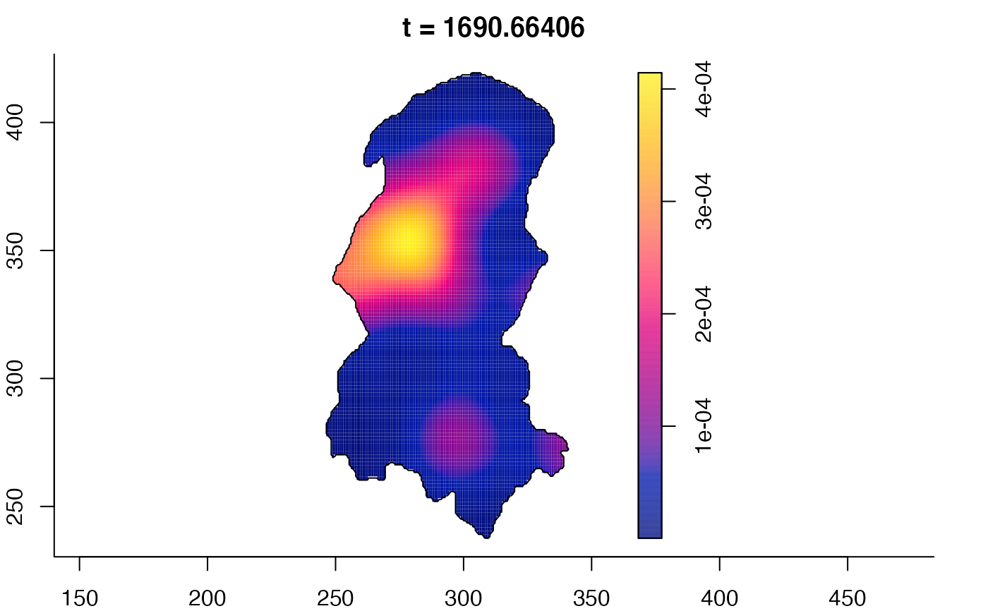
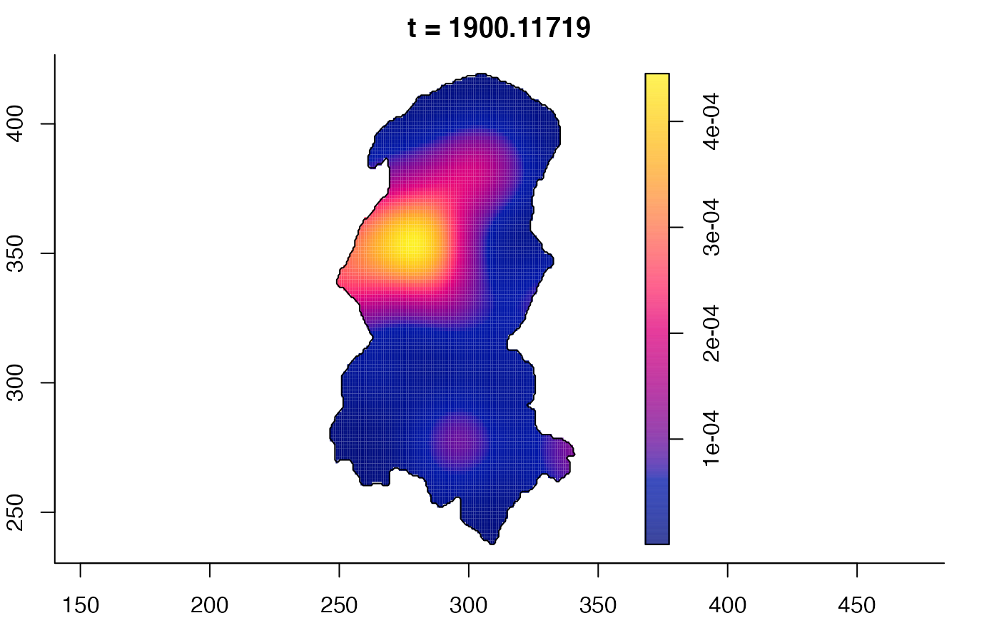
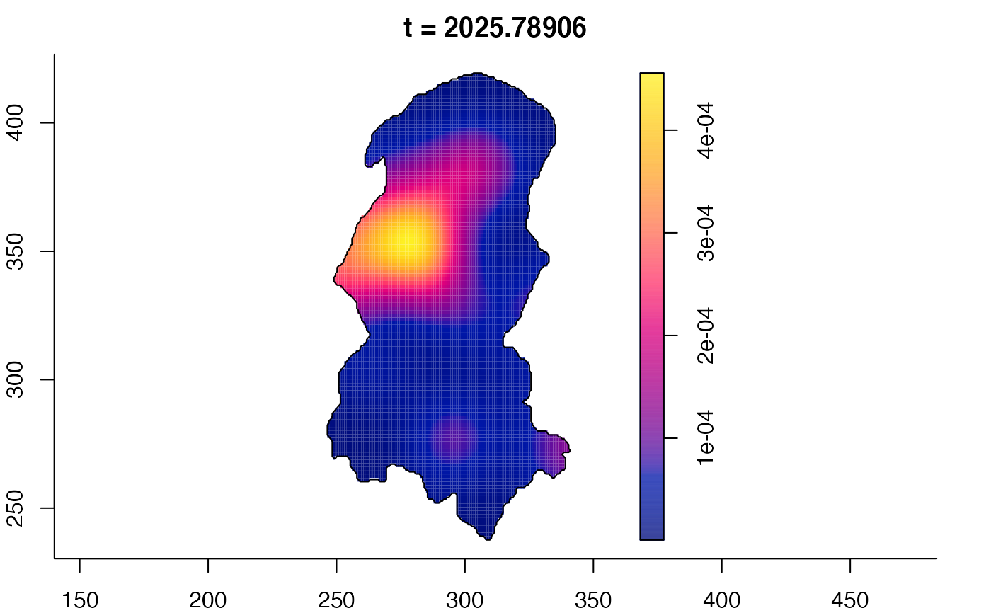
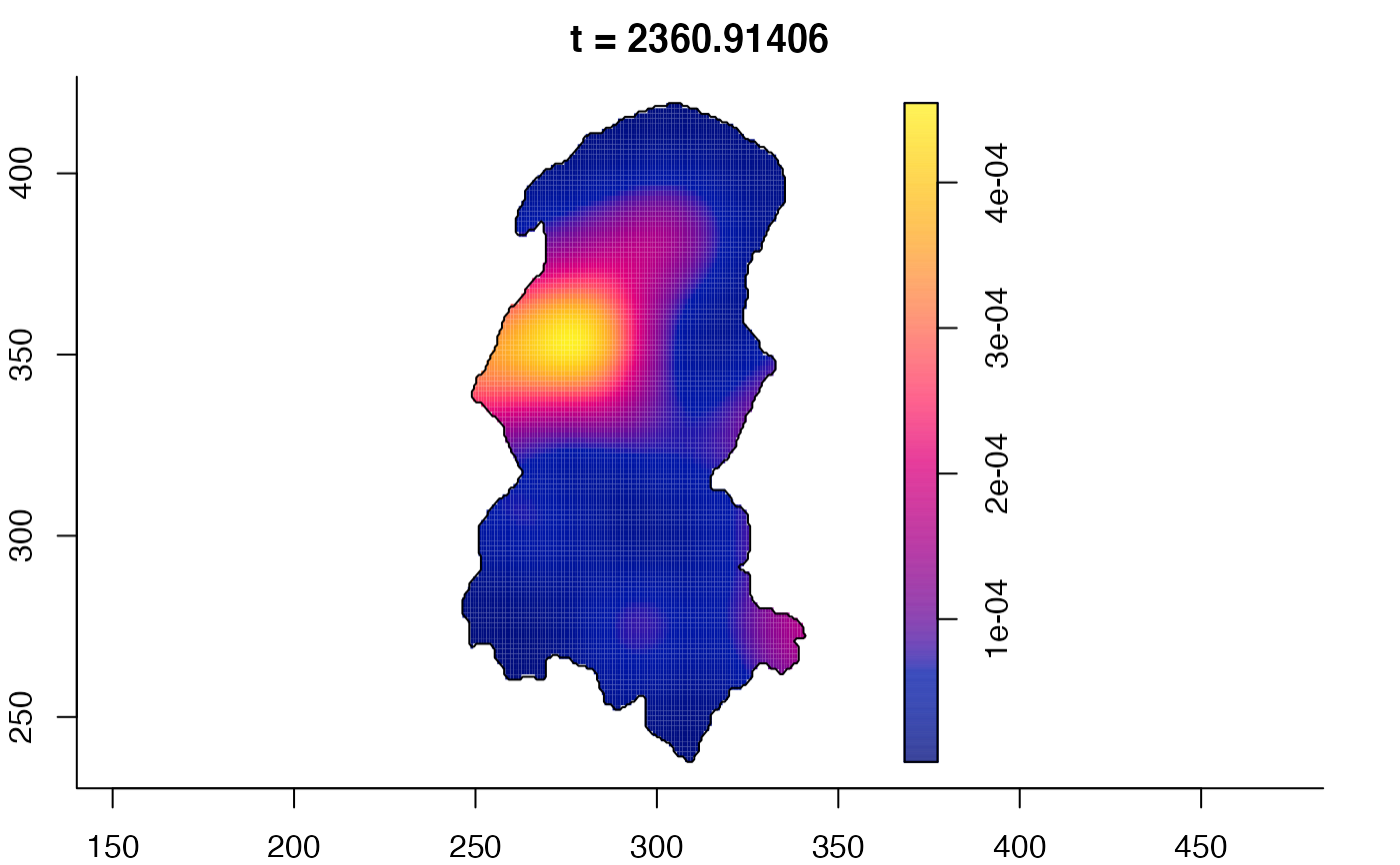
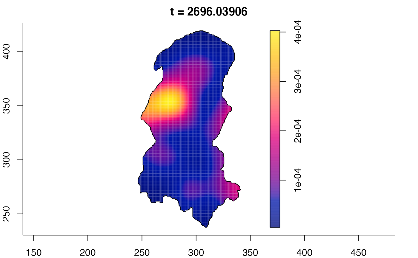
burkden <- spattemp.density(burk$cases,tres=128) # observation times are stored in marks(burk$cases)
#> Calculating trivariate smooth...
#> Done.
#> Edge-correcting...
#> Done.
#> Conditioning on time...
#> Done.
plot(burkden,fix.range=TRUE,sleep=0.1) # animation
# 'stden' object
burkden <- spattemp.density(burk$cases,tres=128) # observation times are stored in marks(burk$cases)
#> Calculating trivariate smooth...
#> Done.
#> Edge-correcting...
#> Done.
#> Conditioning on time...
#> Done.
plot(burkden,fix.range=TRUE,sleep=0.1) # animation


 plot(burkden,tselect=c(1000,3000),type="conditional") # spatial densities conditional on each time


 # 'rrs' object
pbcrr <- risk(pbc,h0=4,hp=3,adapt=TRUE,tolerate=TRUE,davies.baddeley=0.025,edge="diggle")
#> Estimating case density...
#> Done.
#> Estimating control density...
#> Done.
#> Calculating tolerance contours...
#> Done.
plot(pbcrr) # default
# 'rrs' object
pbcrr <- risk(pbc,h0=4,hp=3,adapt=TRUE,tolerate=TRUE,davies.baddeley=0.025,edge="diggle")
#> Estimating case density...
#> Done.
#> Estimating control density...
#> Done.
#> Calculating tolerance contours...
#> Done.
plot(pbcrr) # default
 plot(pbcrr,tol.args=list(levels=c(0.05,0.01),lty=2:1,col="seagreen4"),auto.axes=FALSE)
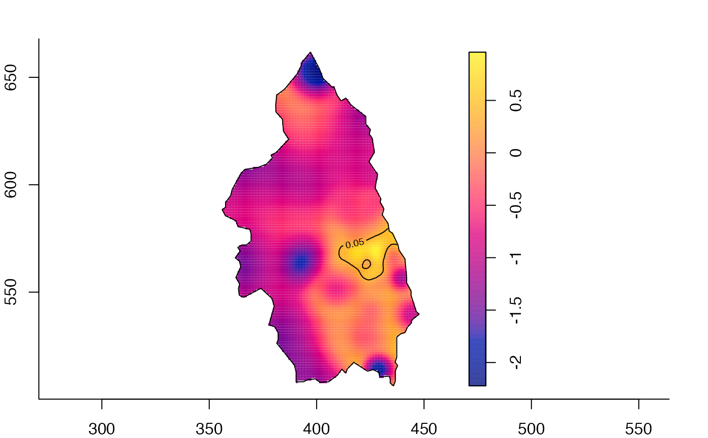
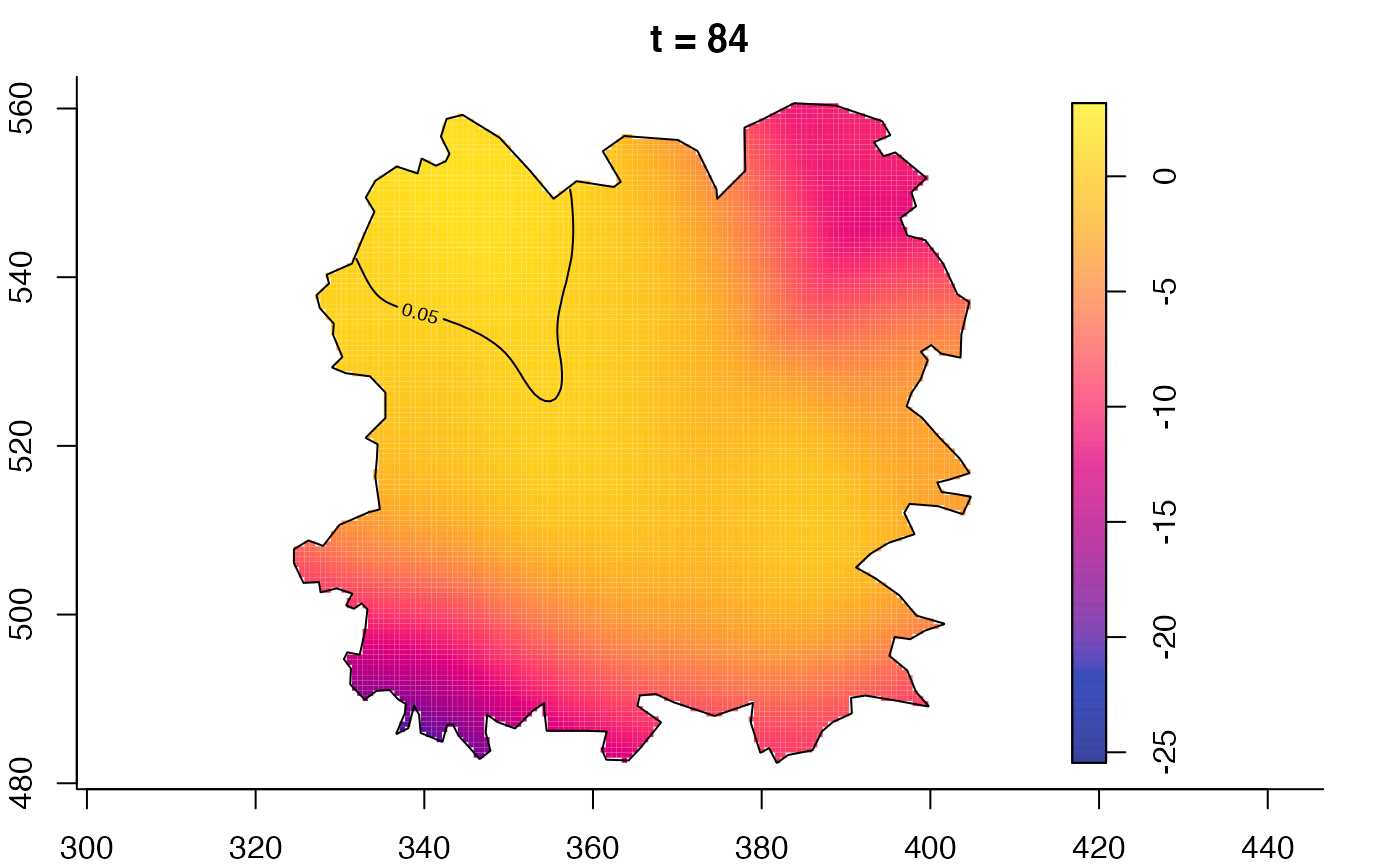
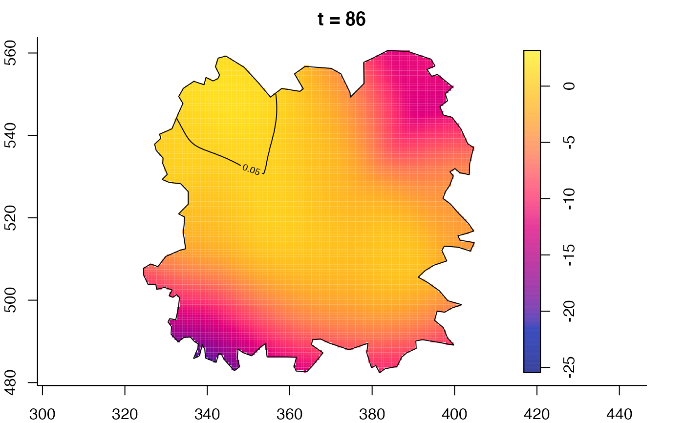
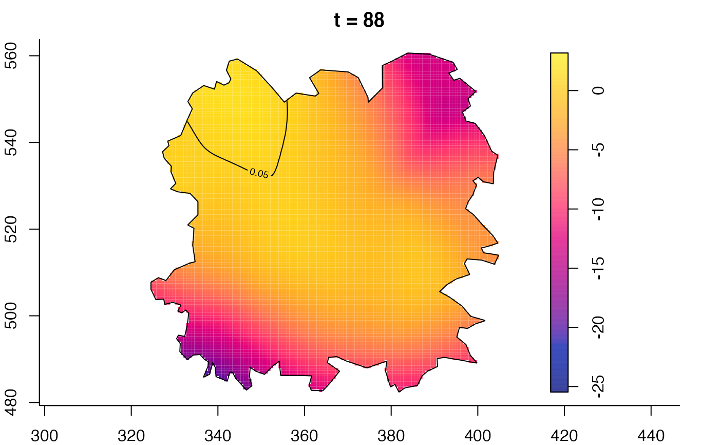
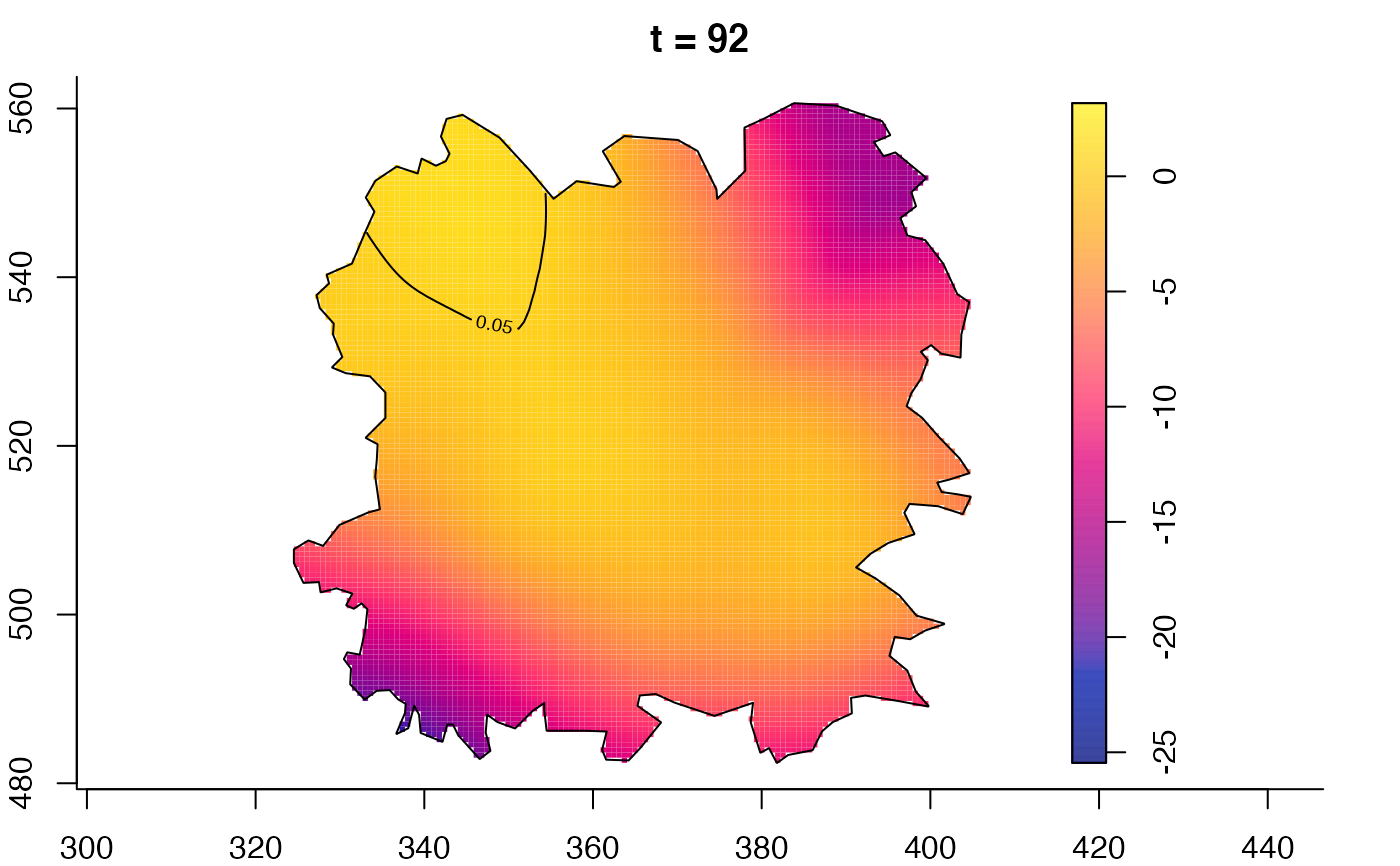
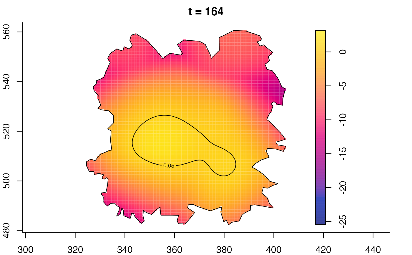
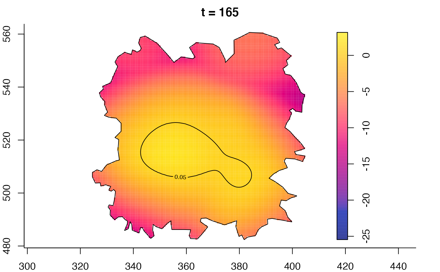
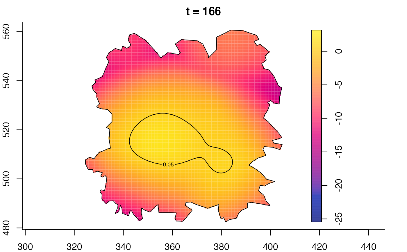
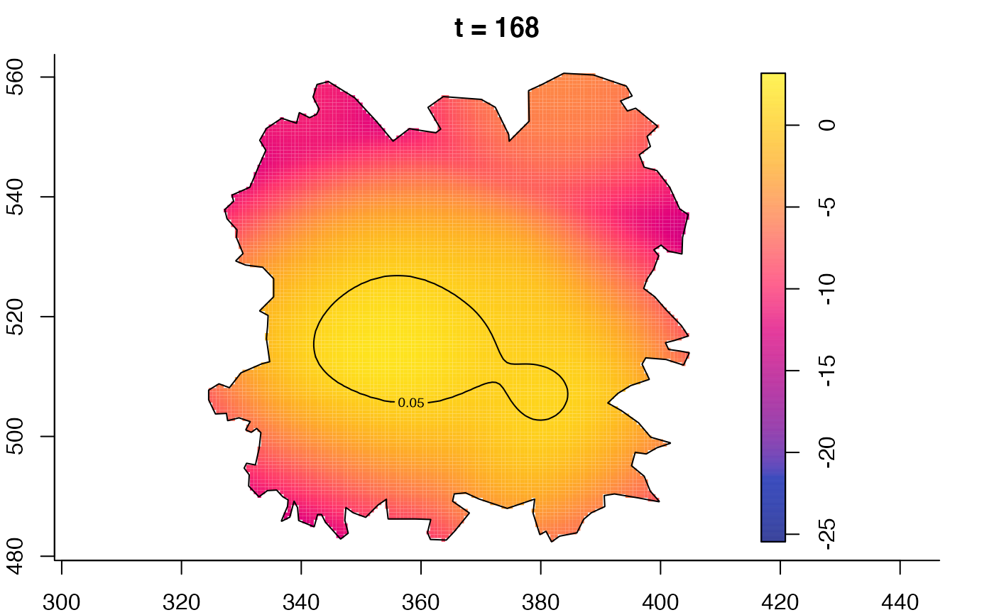
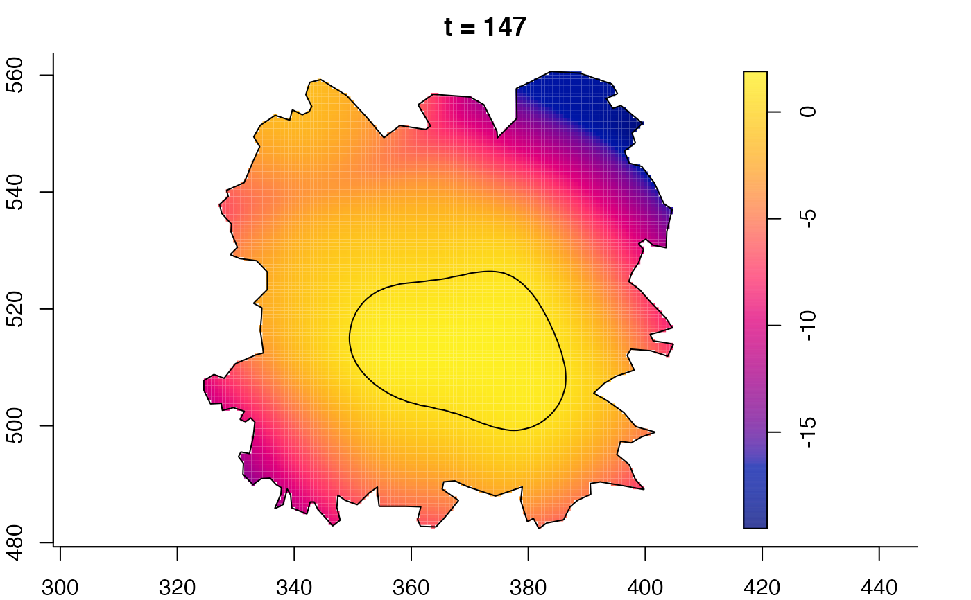
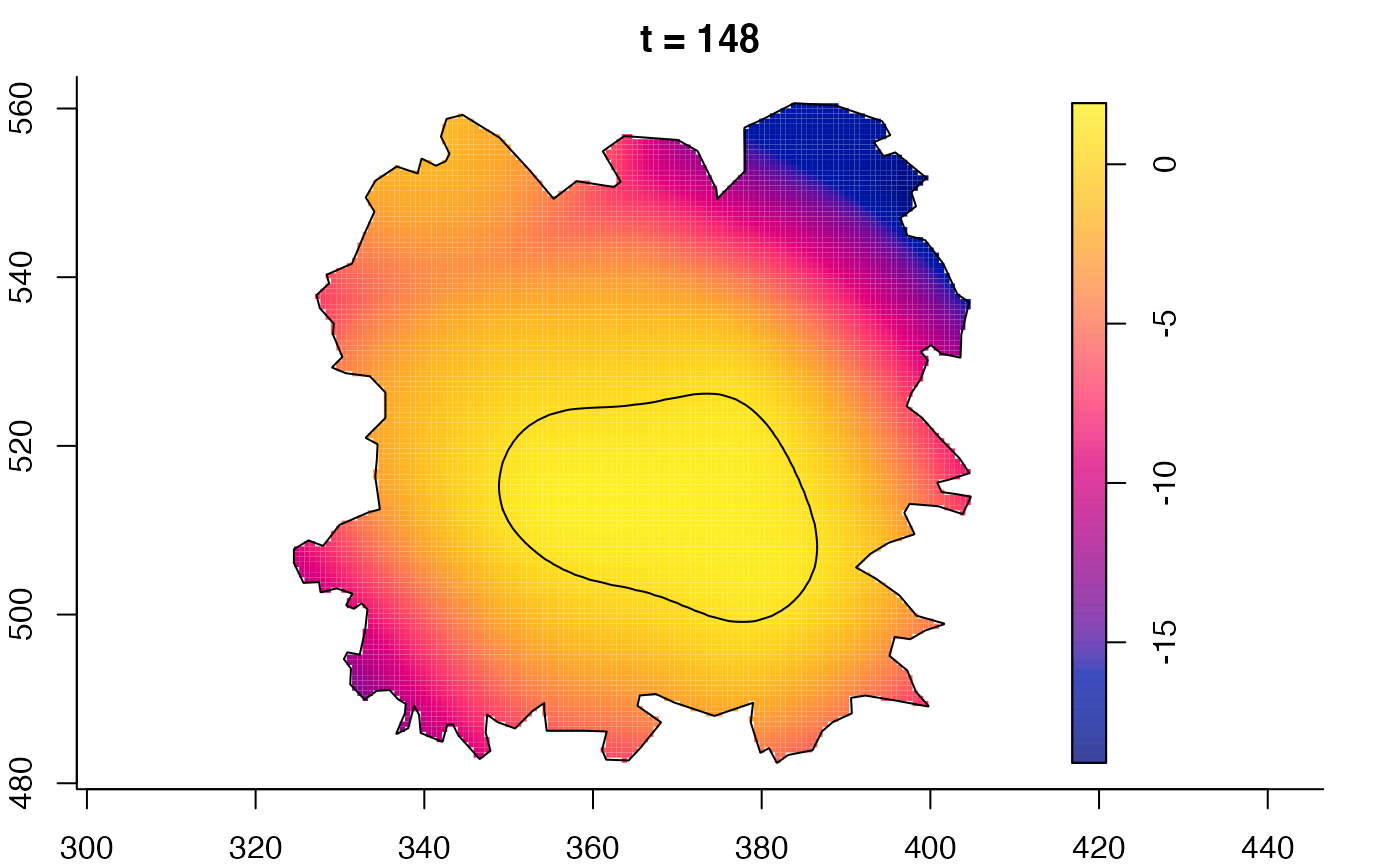
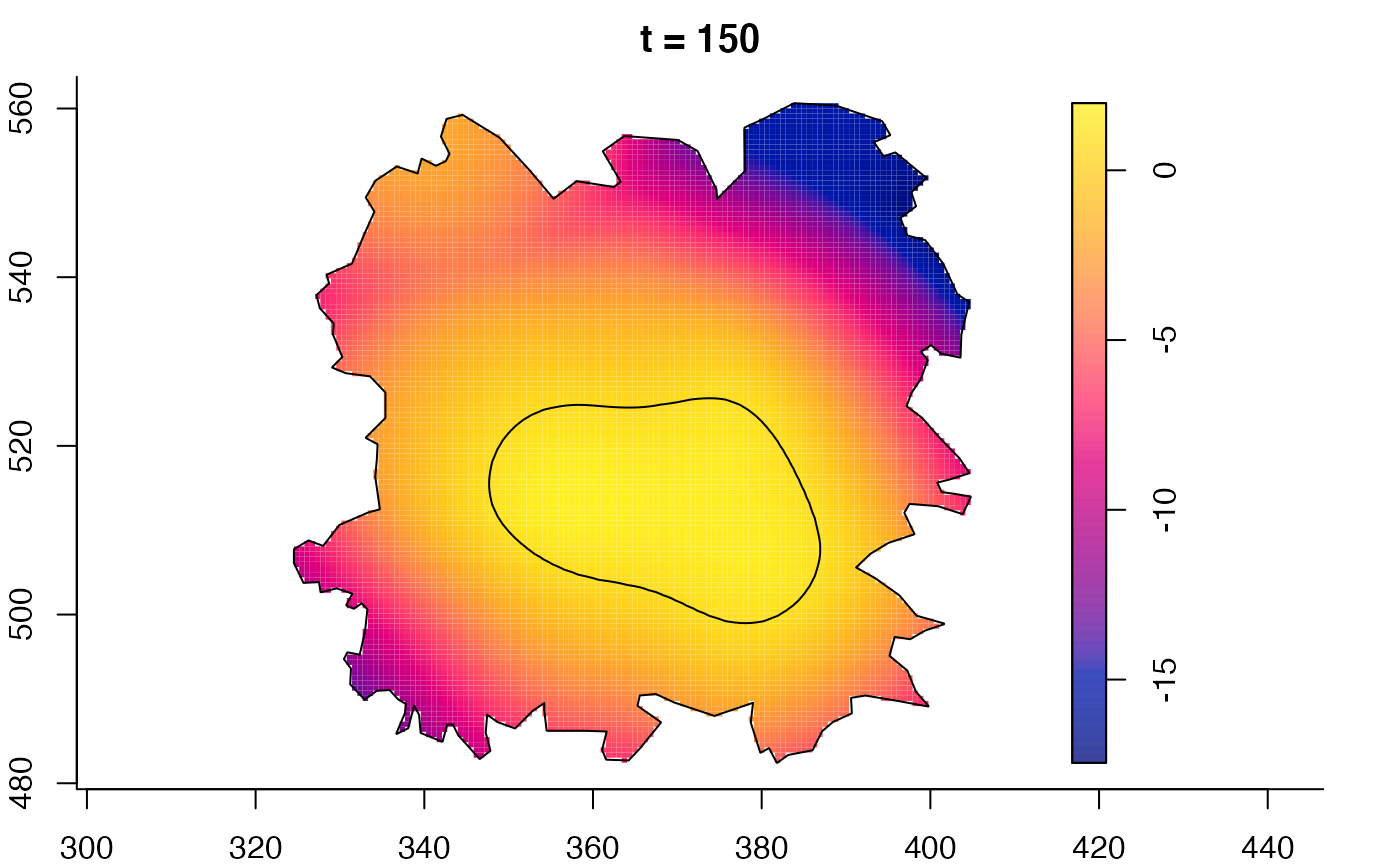
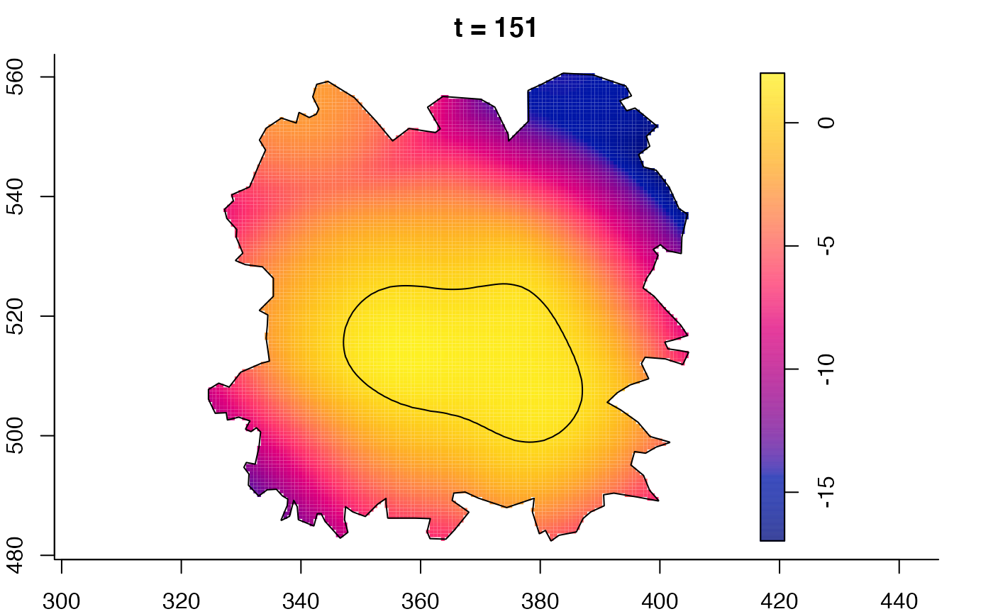
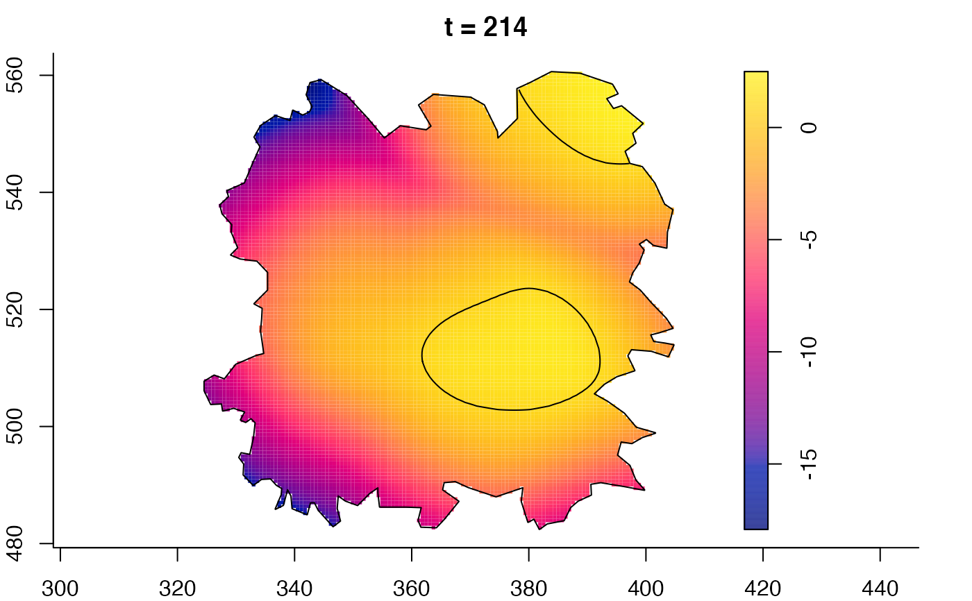
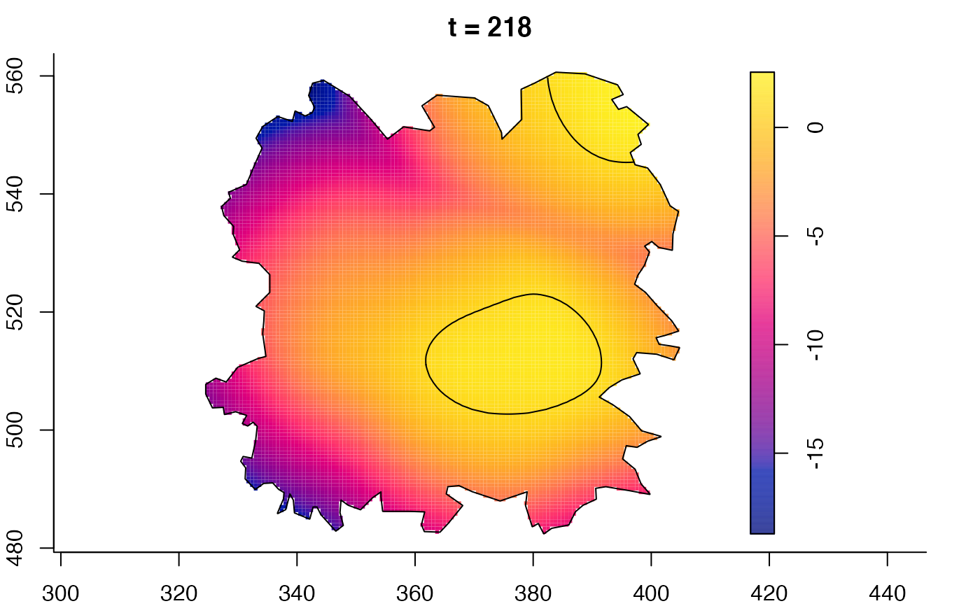
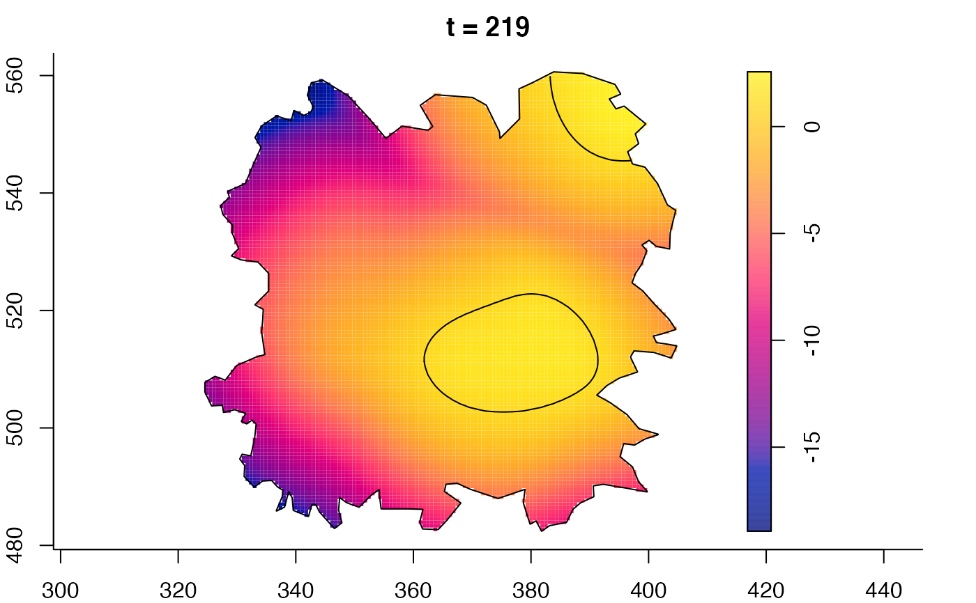
 # 'rrst' object
f <- spattemp.density(fmd$cases,h=6,lambda=8)
#> Calculating trivariate smooth...
#> Done.
#> Edge-correcting...
#> Done.
#> Conditioning on time...
#> Done.
g <- bivariate.density(fmd$controls,h0=6)
fmdrr <- spattemp.risk(f,g,tolerate=TRUE)
#> Calculating ratio...
#> Done.
#> Ensuring finiteness...
#> --joint--
#> --conditional--
#> Done.
#> Calculating tolerance contours...
#> --convolution 1--
#> --convolution 2--
#> Done.
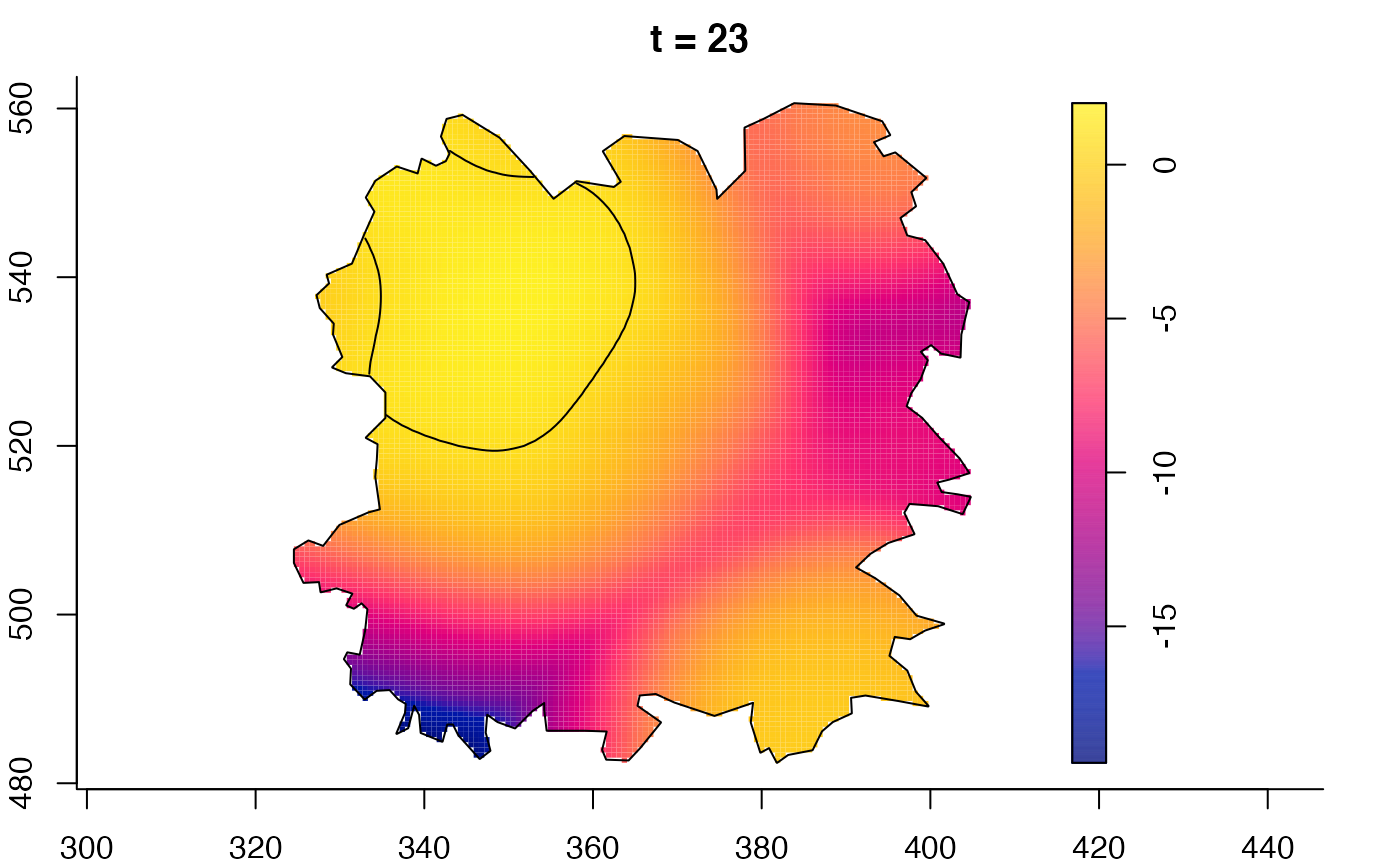
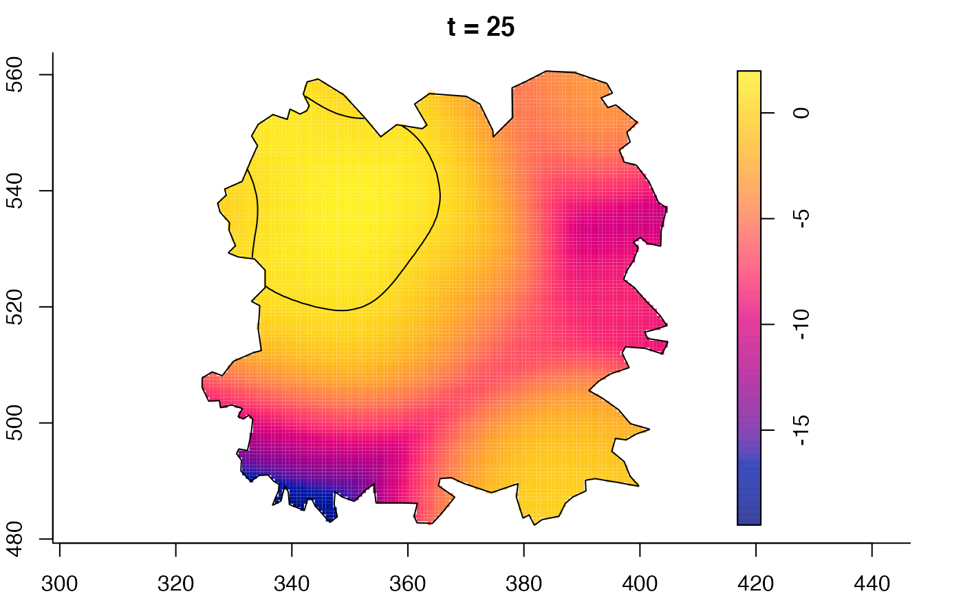
plot(fmdrr,sleep=0.1,fix.range=TRUE)
# 'rrst' object
f <- spattemp.density(fmd$cases,h=6,lambda=8)
#> Calculating trivariate smooth...
#> Done.
#> Edge-correcting...
#> Done.
#> Conditioning on time...
#> Done.
g <- bivariate.density(fmd$controls,h0=6)
fmdrr <- spattemp.risk(f,g,tolerate=TRUE)
#> Calculating ratio...
#> Done.
#> Ensuring finiteness...
#> --joint--
#> --conditional--
#> Done.
#> Calculating tolerance contours...
#> --convolution 1--
#> --convolution 2--
#> Done.
plot(fmdrr,sleep=0.1,fix.range=TRUE)

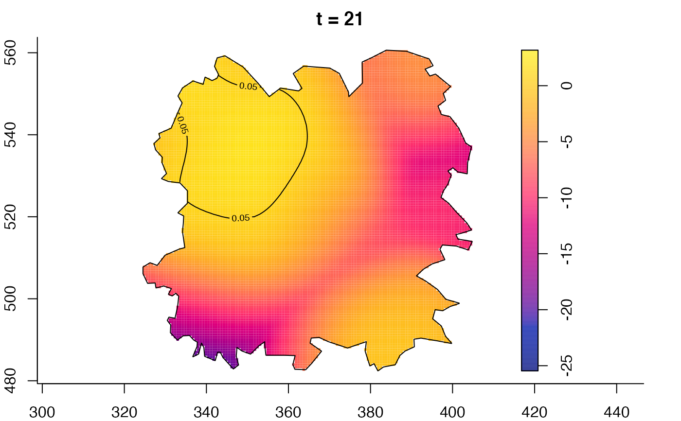
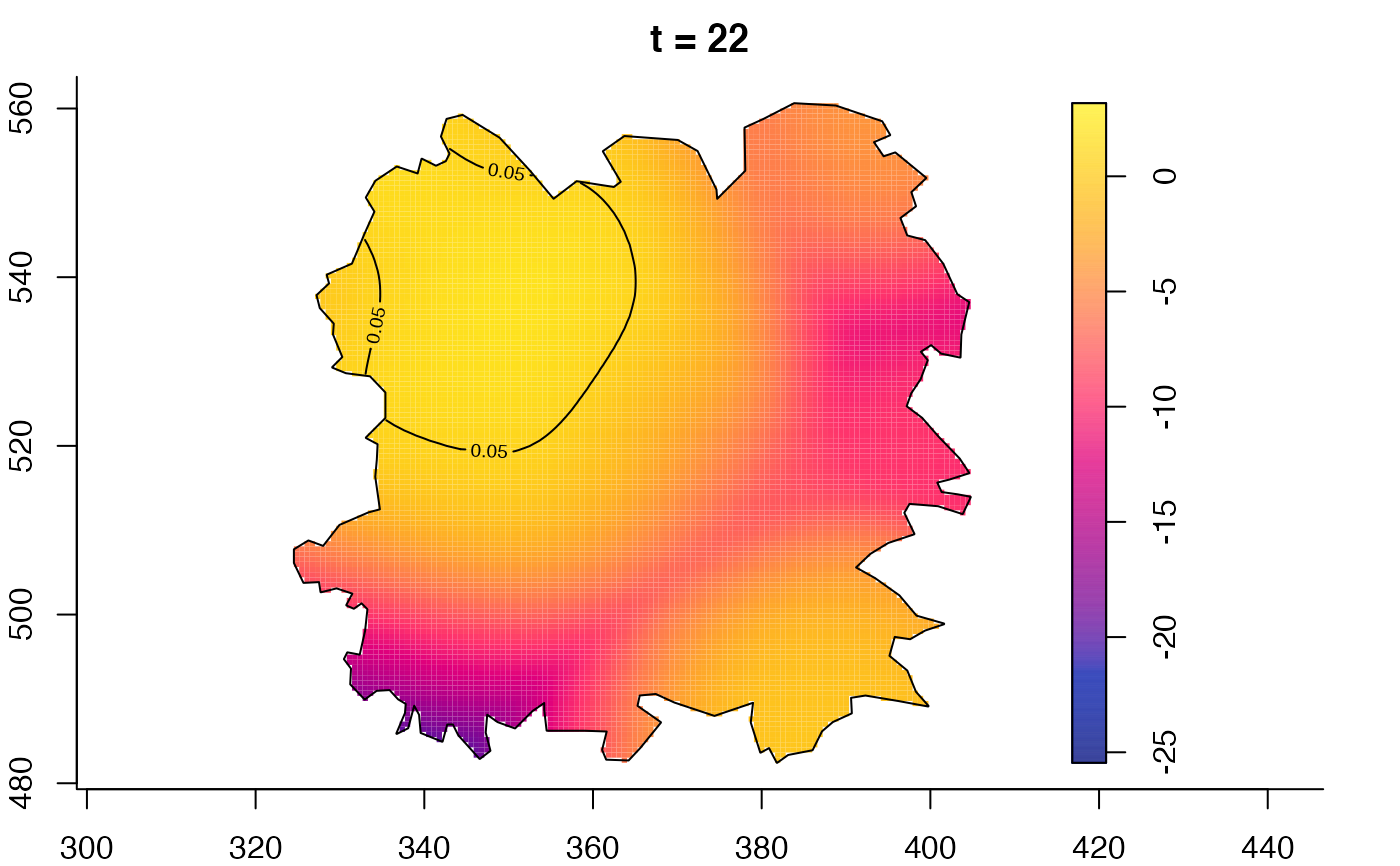

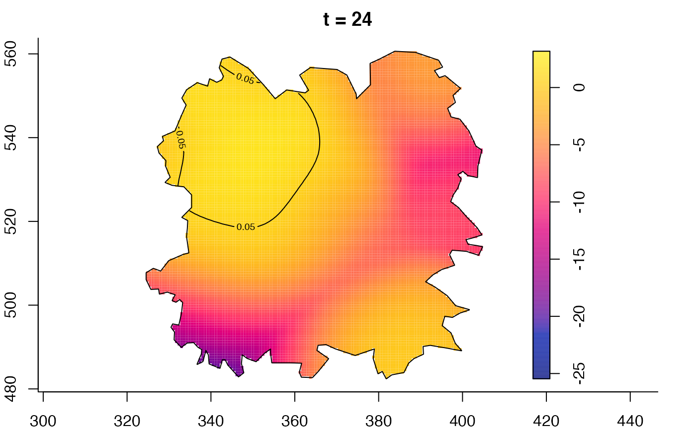


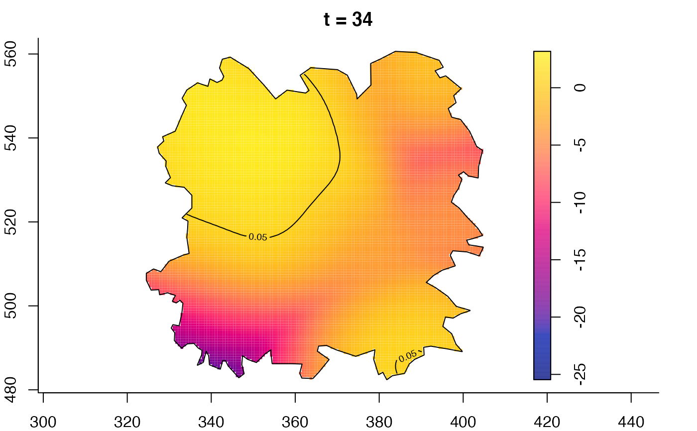


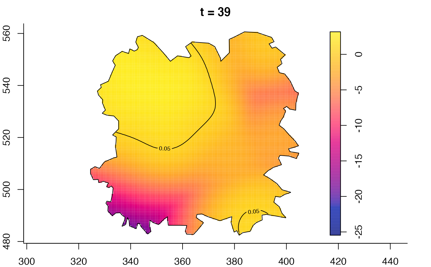


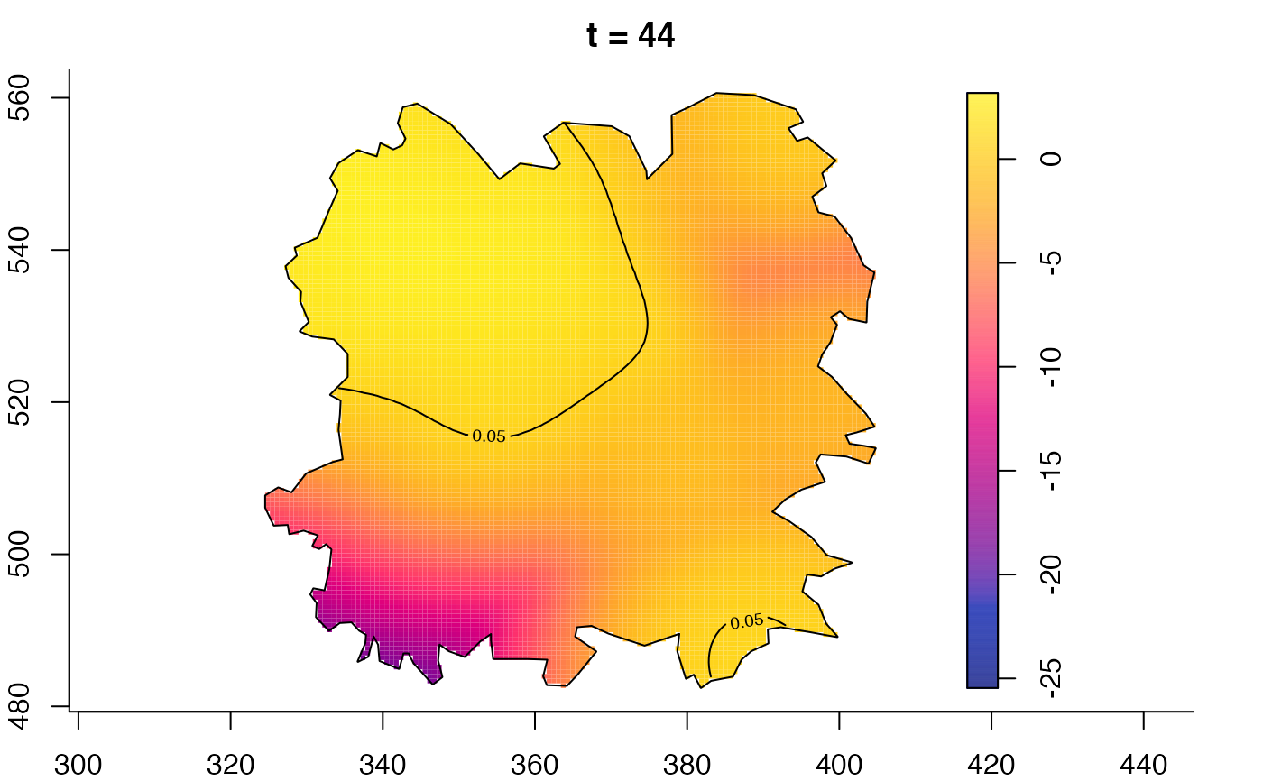


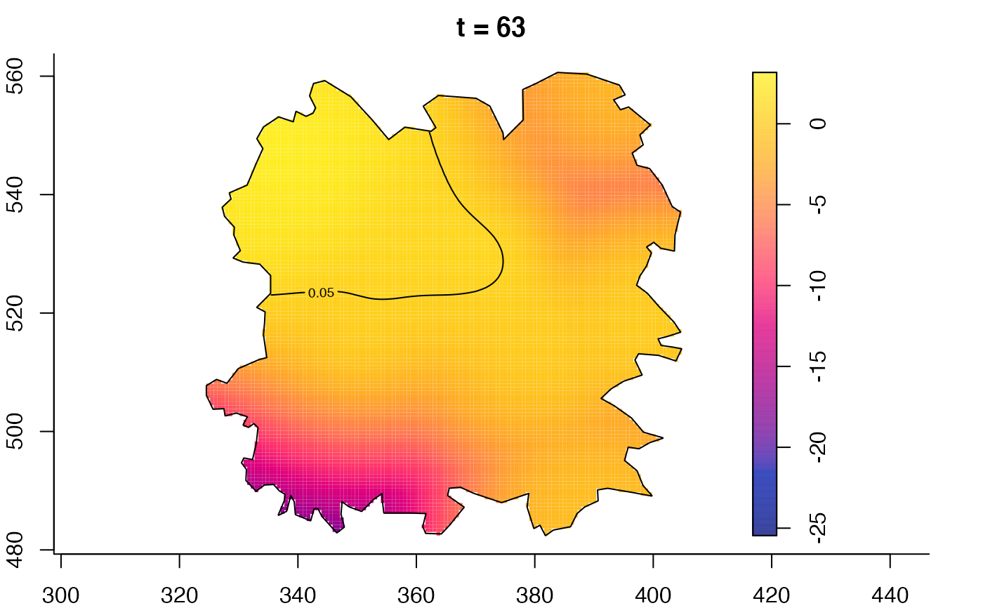


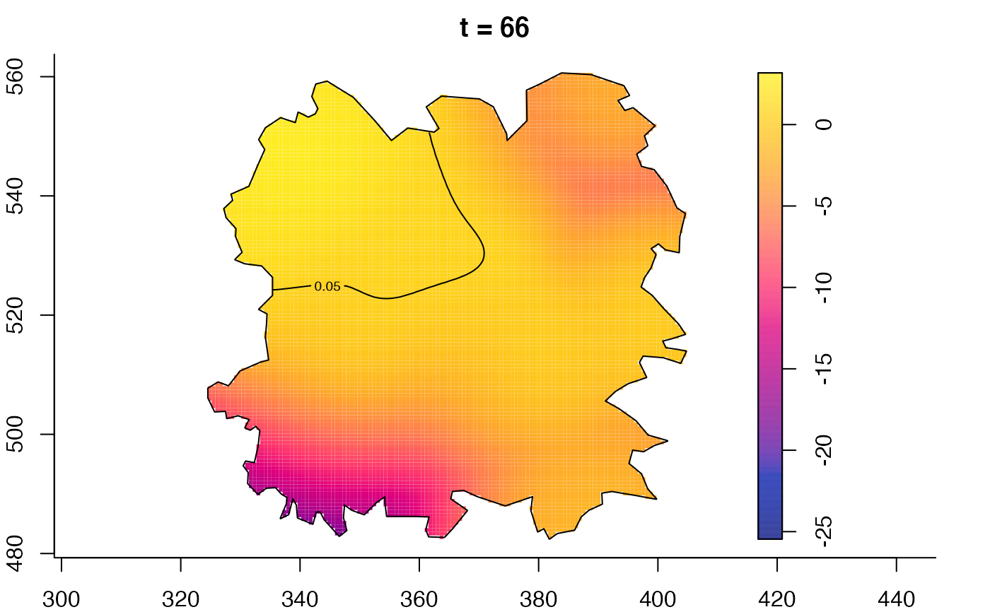


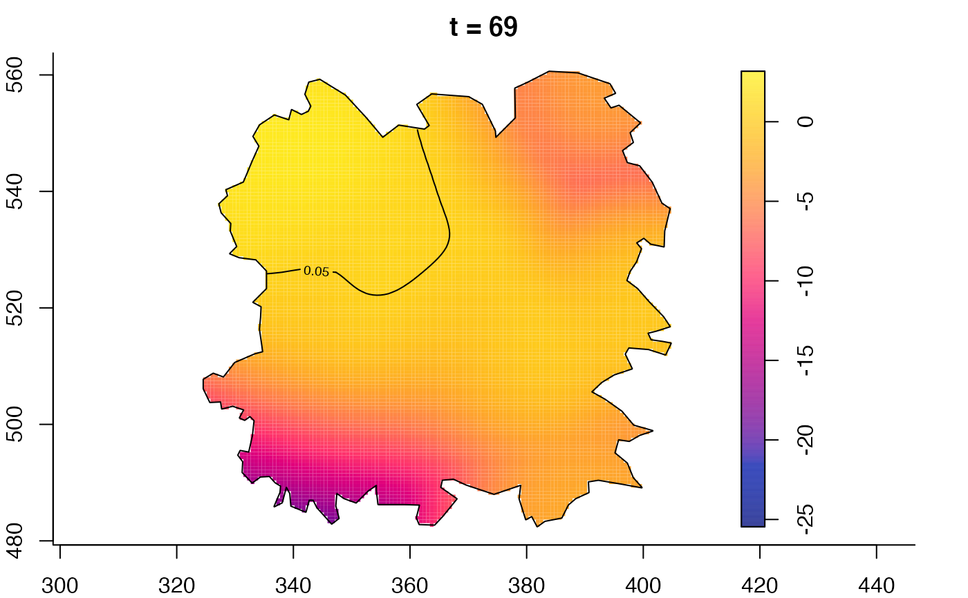


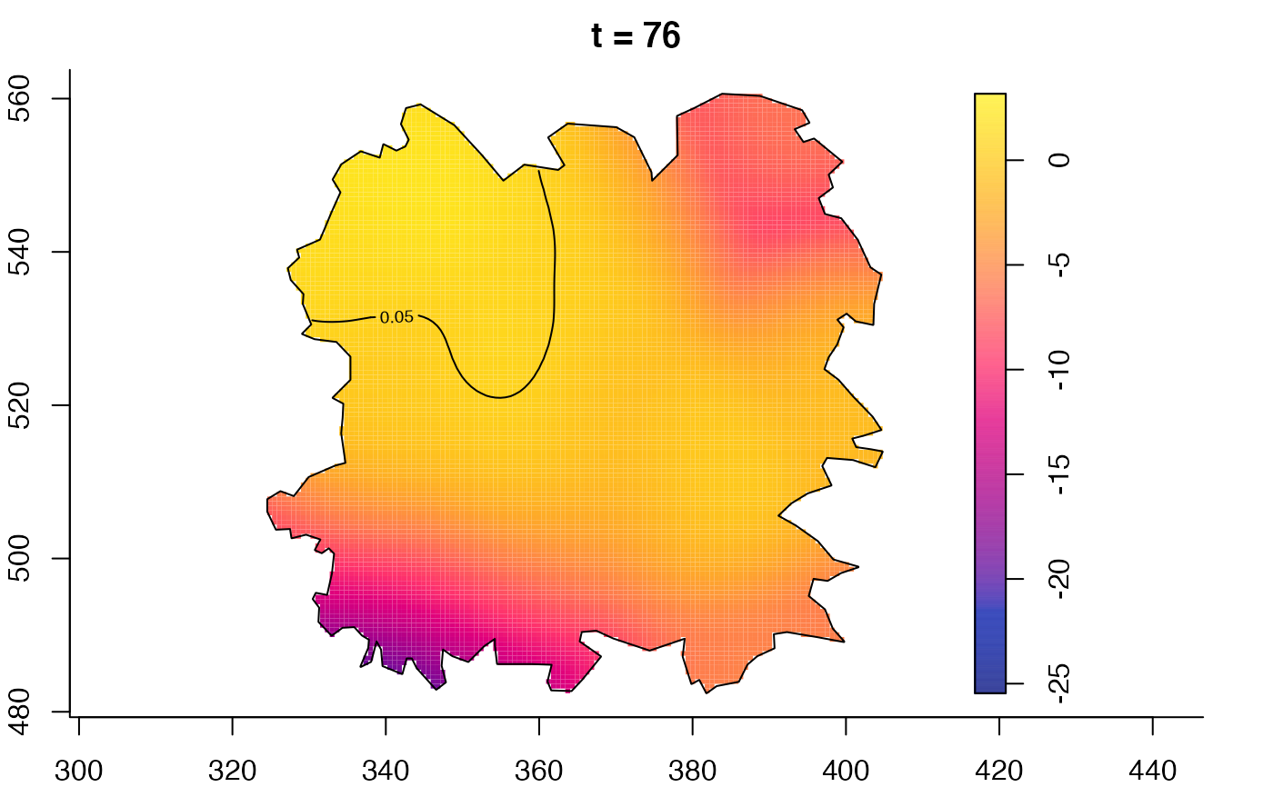


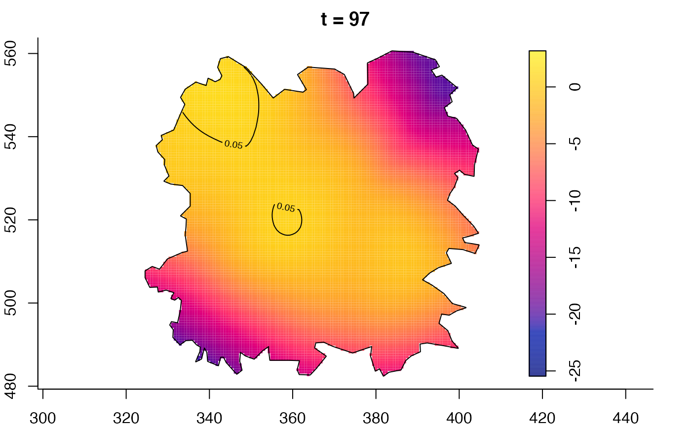


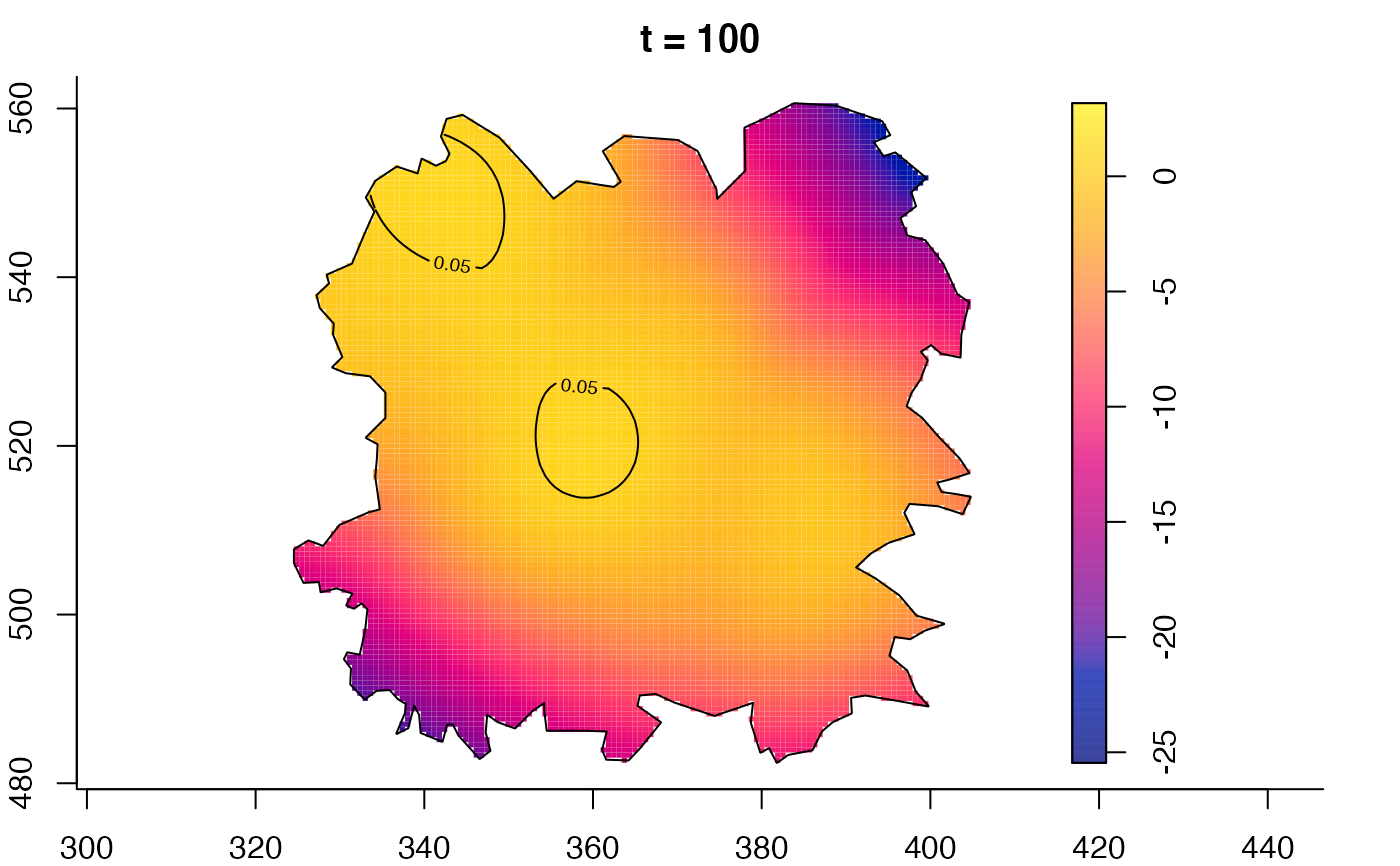


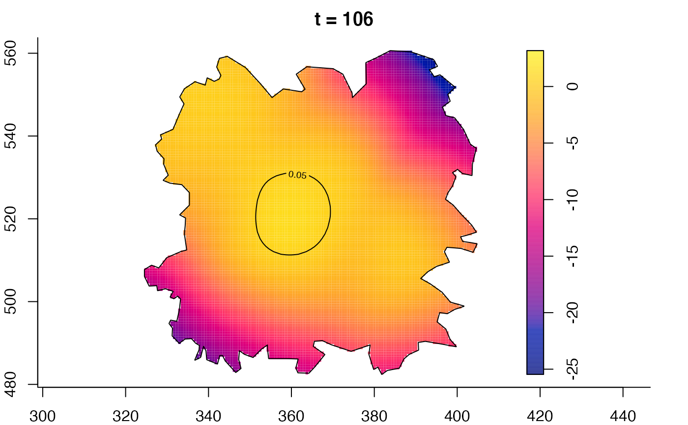


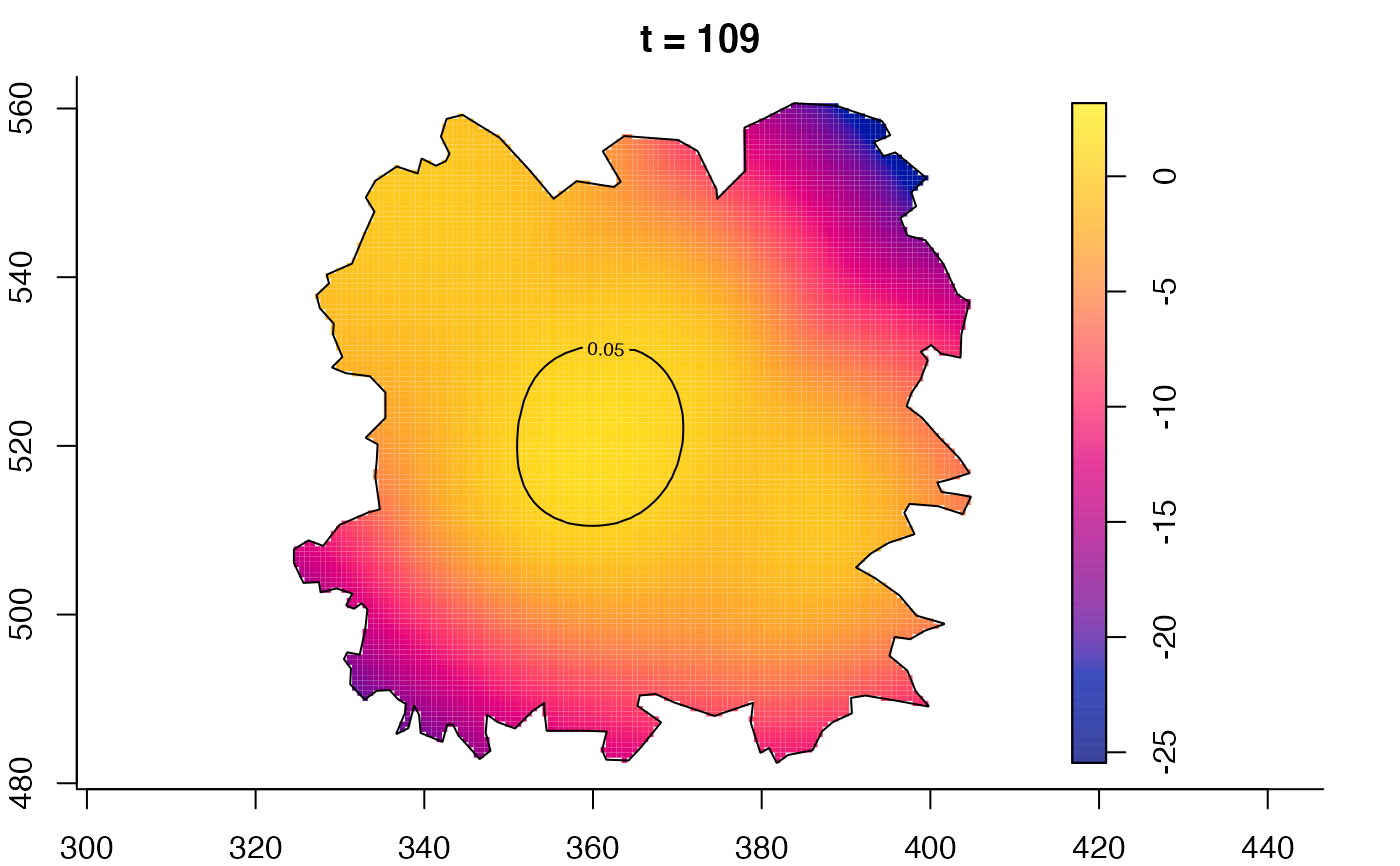


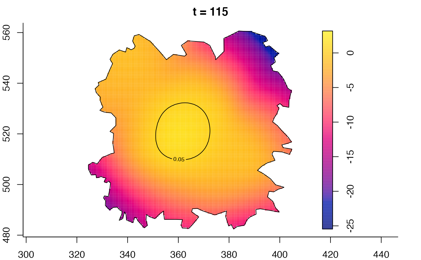


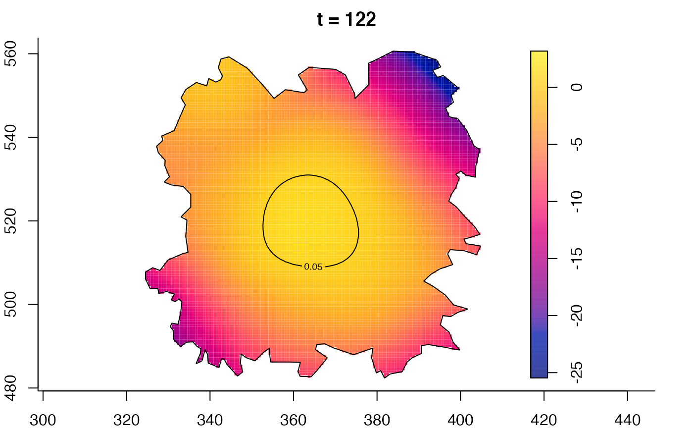

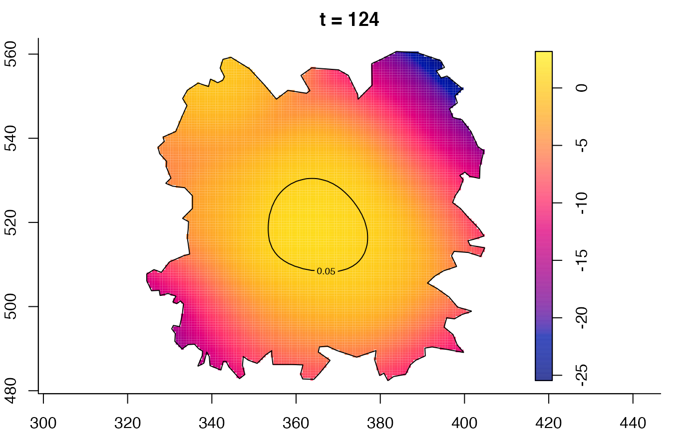
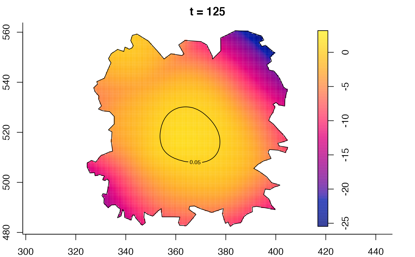


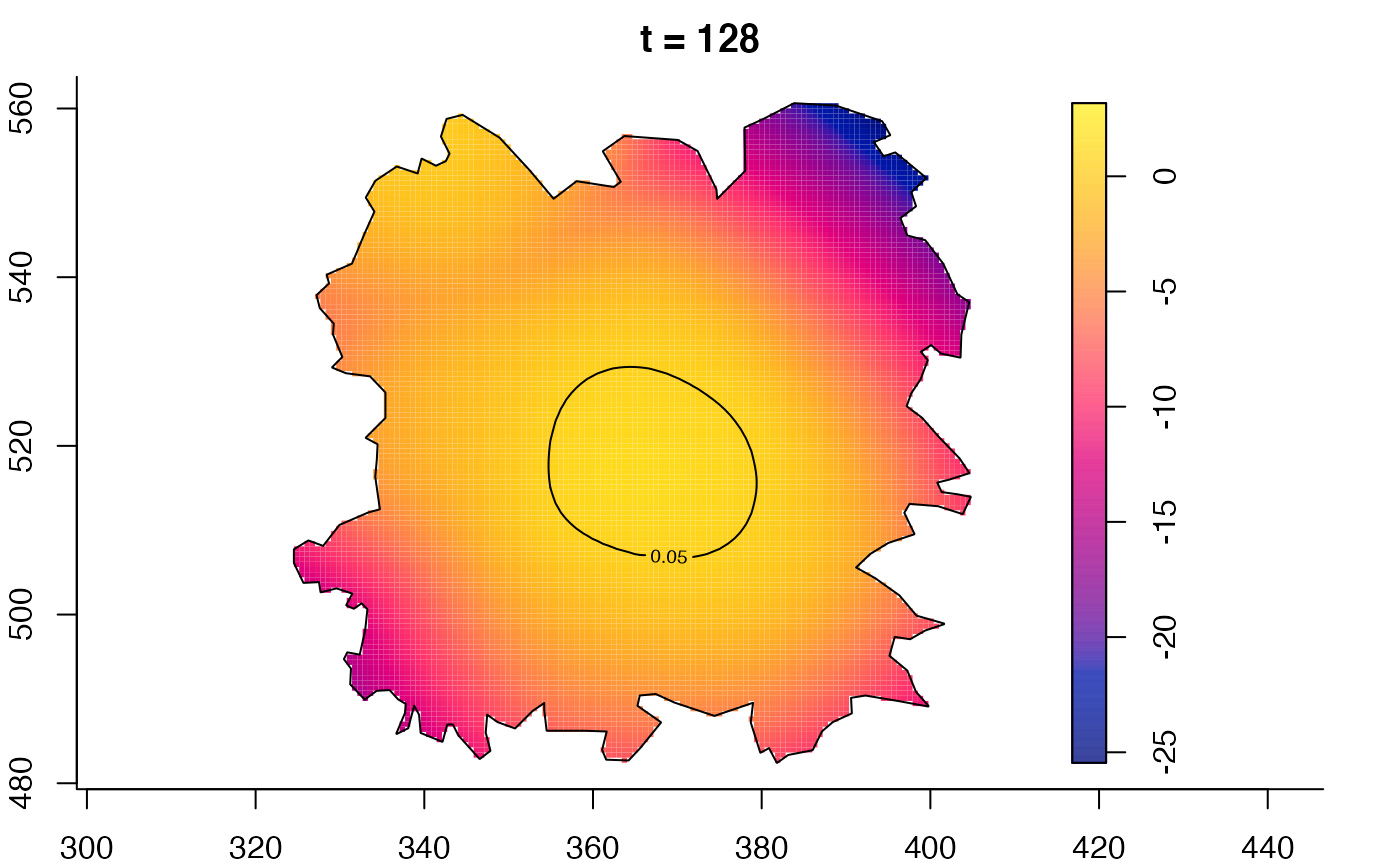

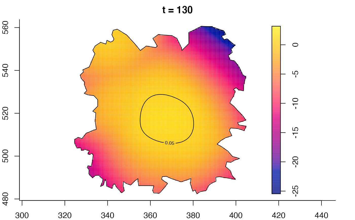


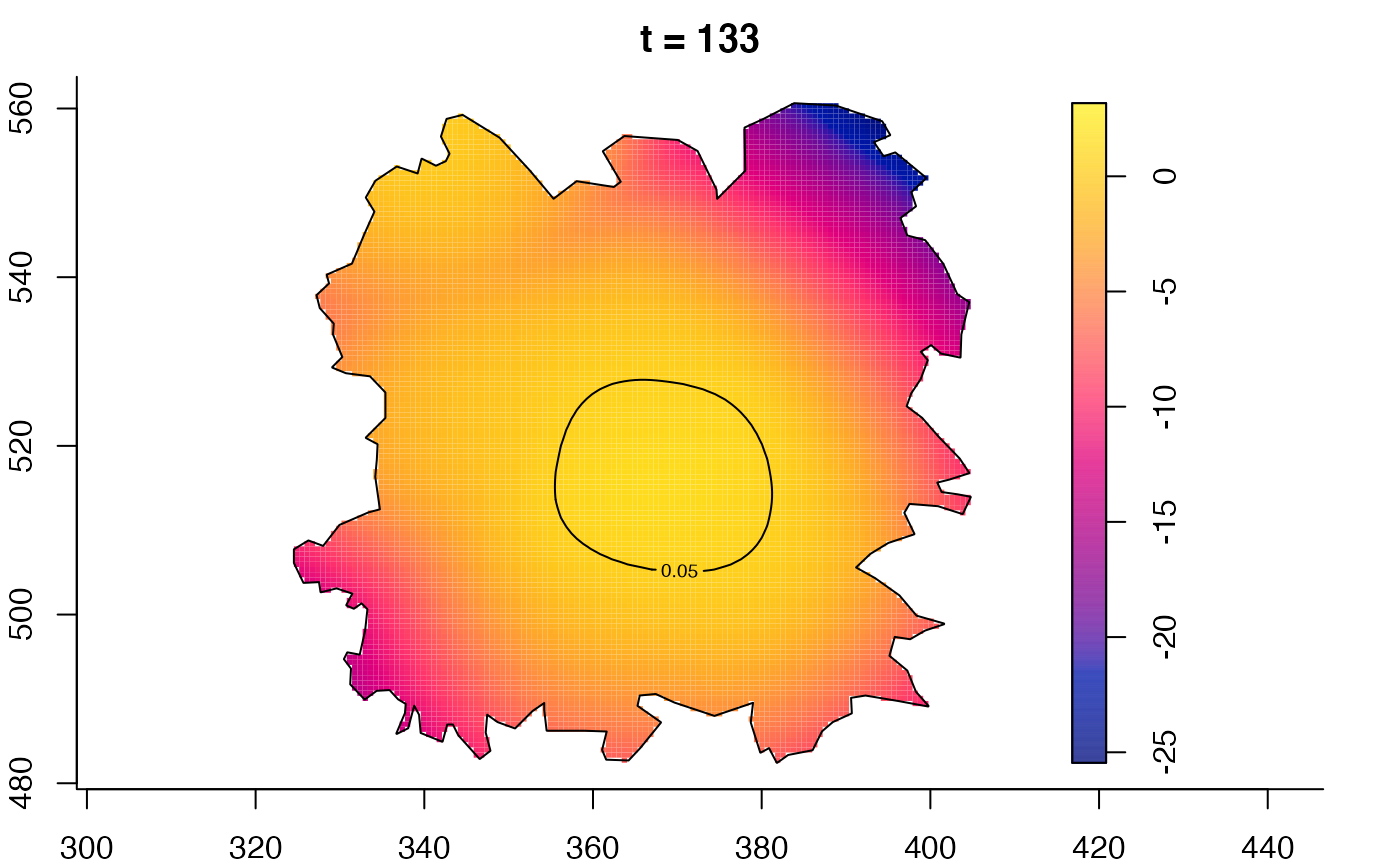


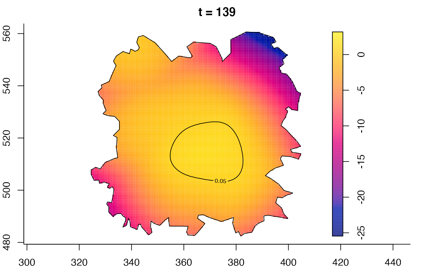


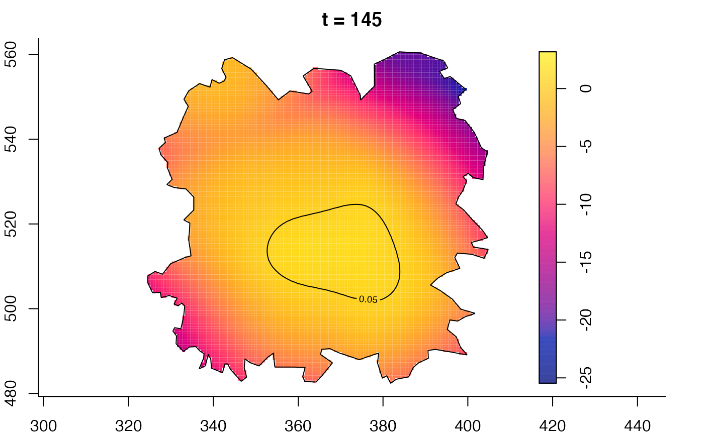


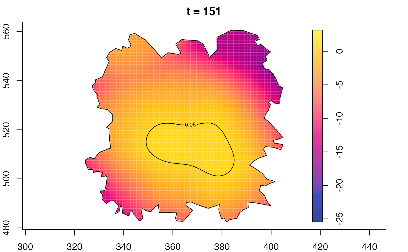


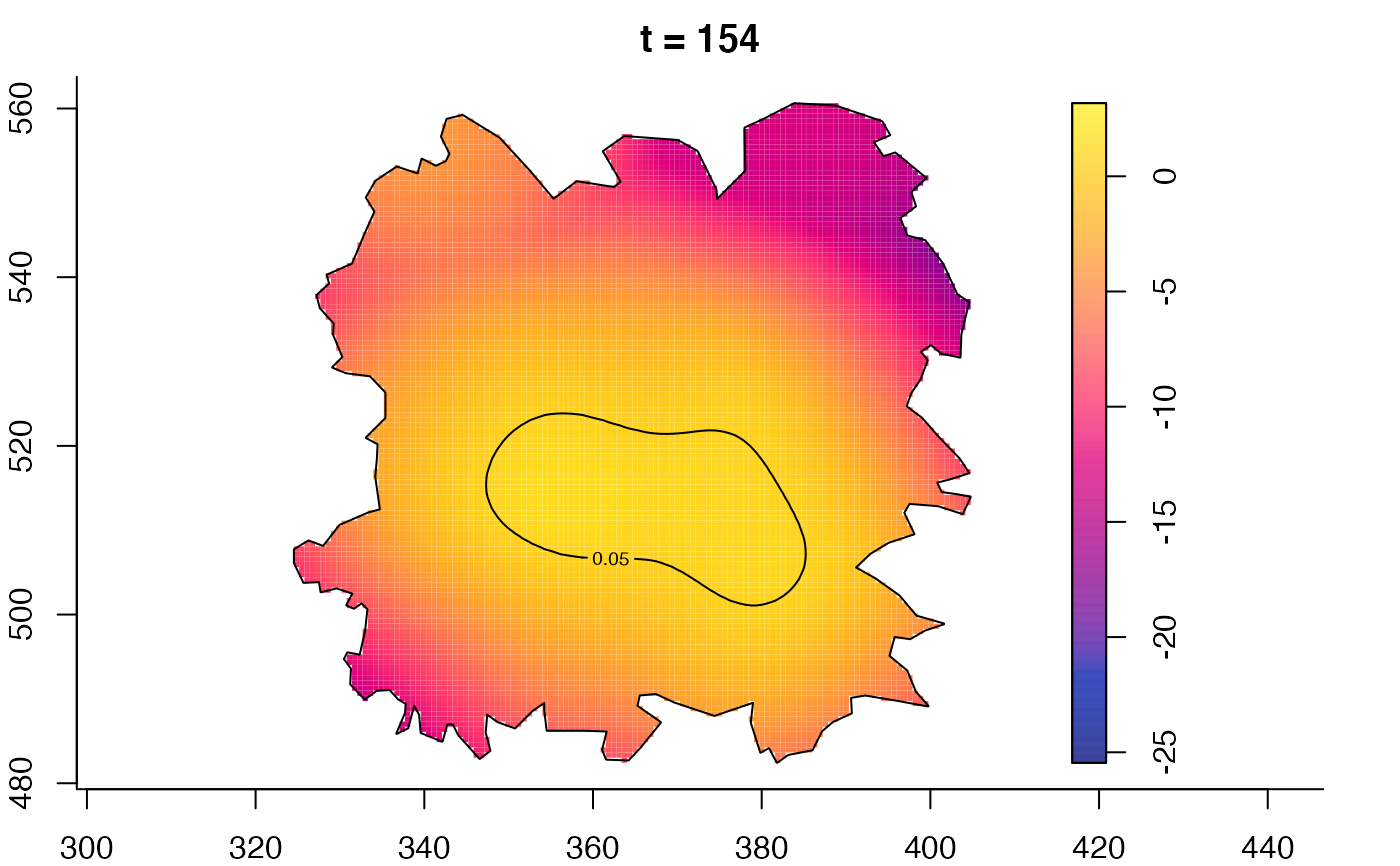

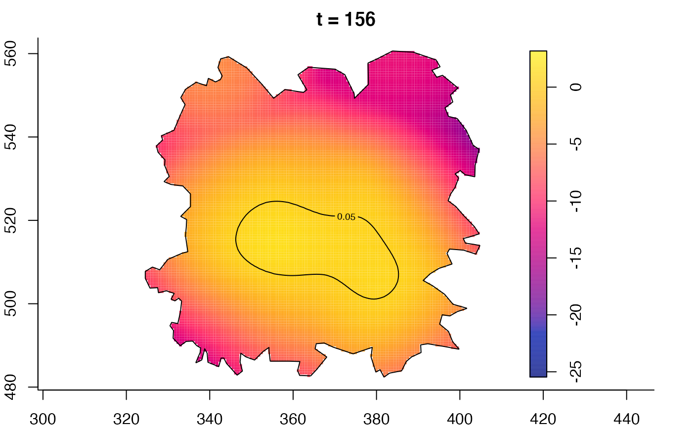
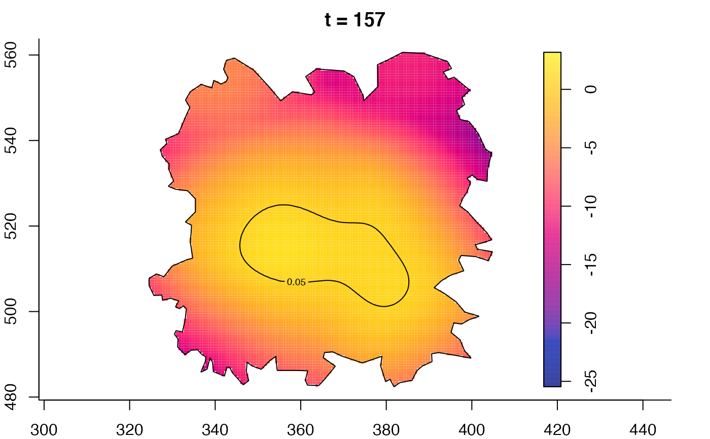
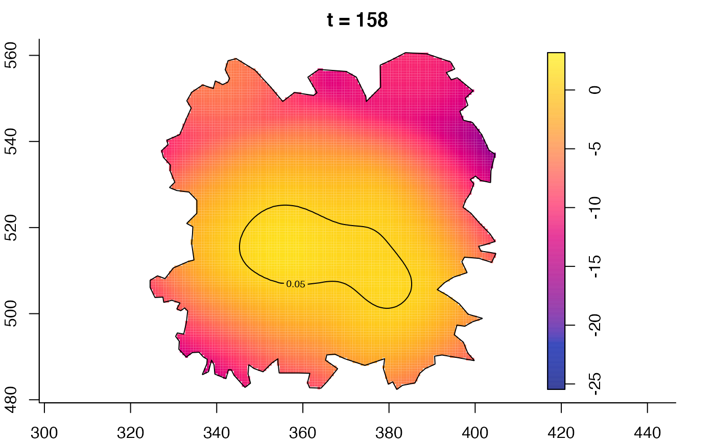
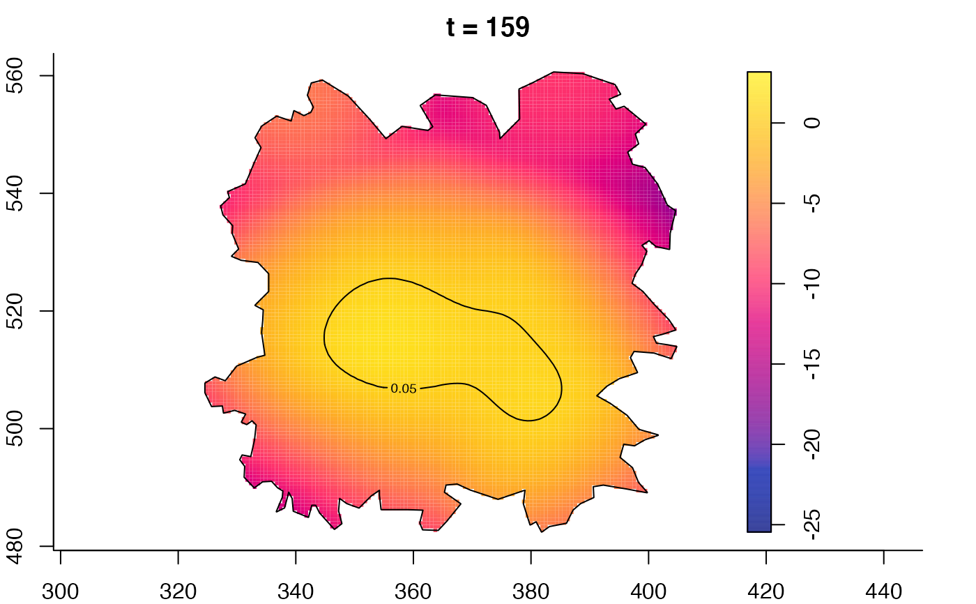

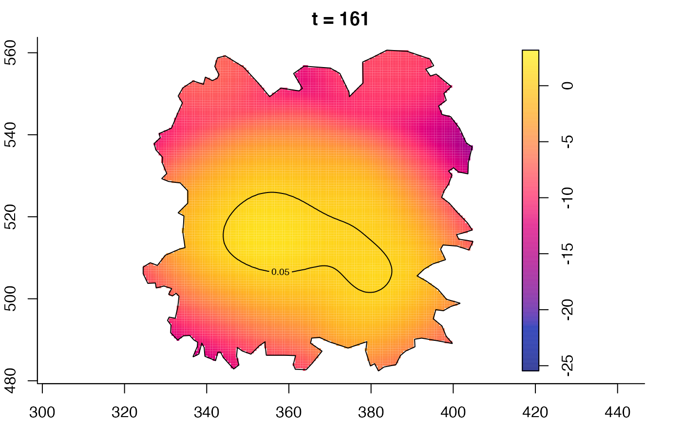


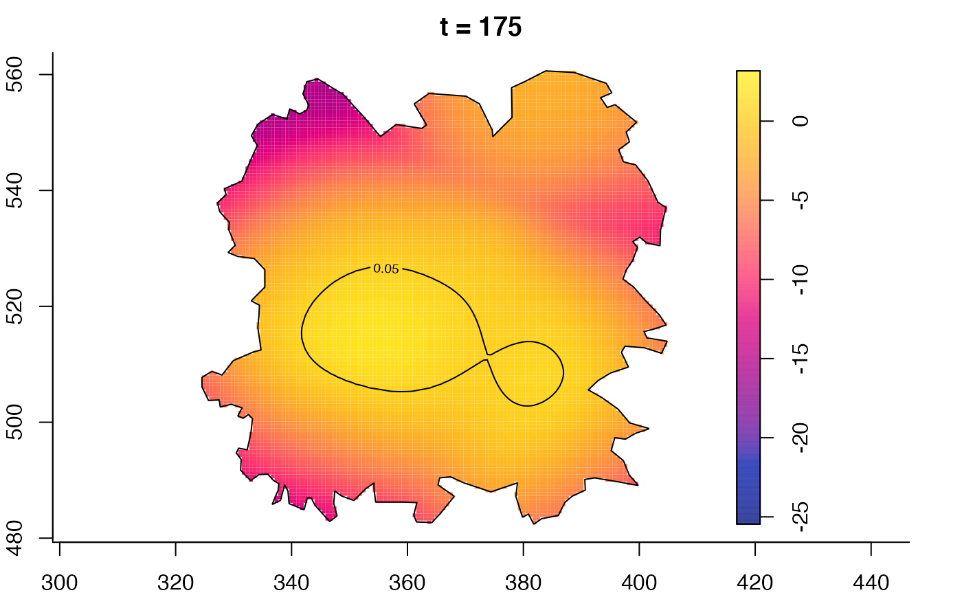
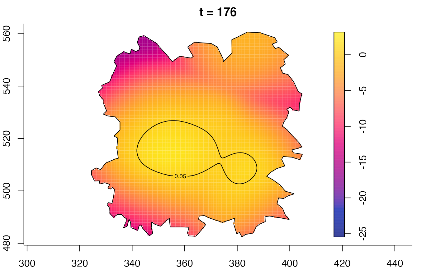


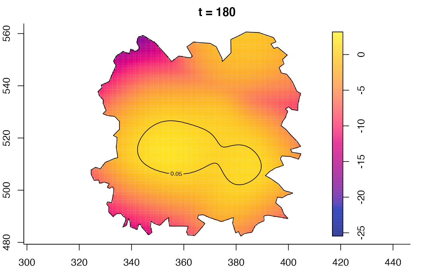


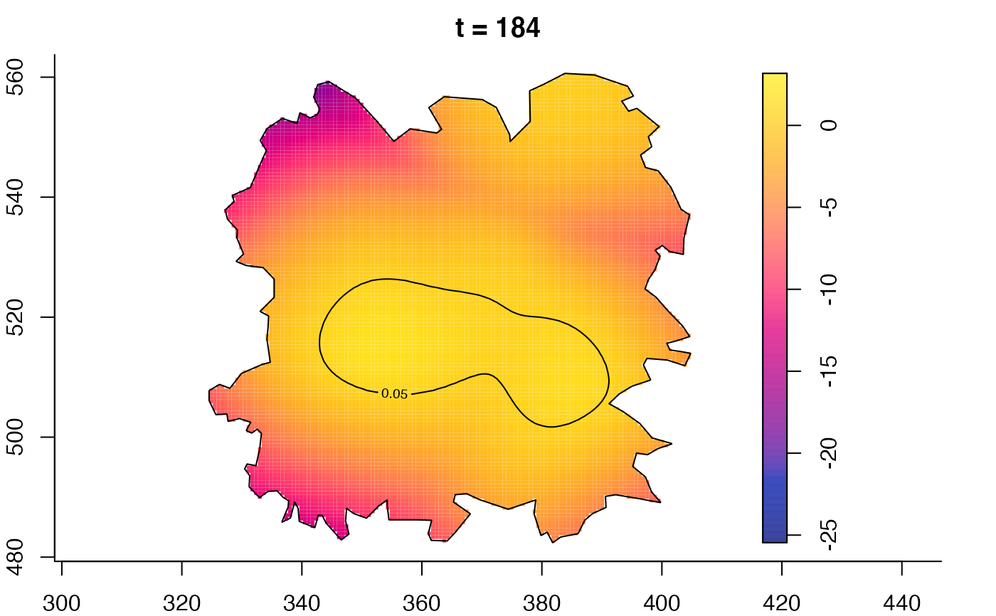


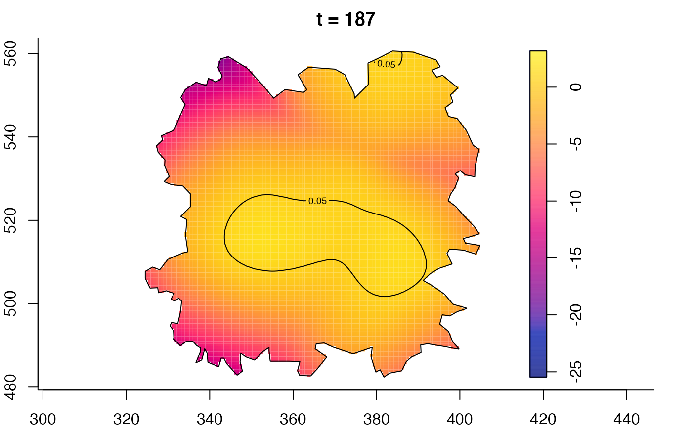


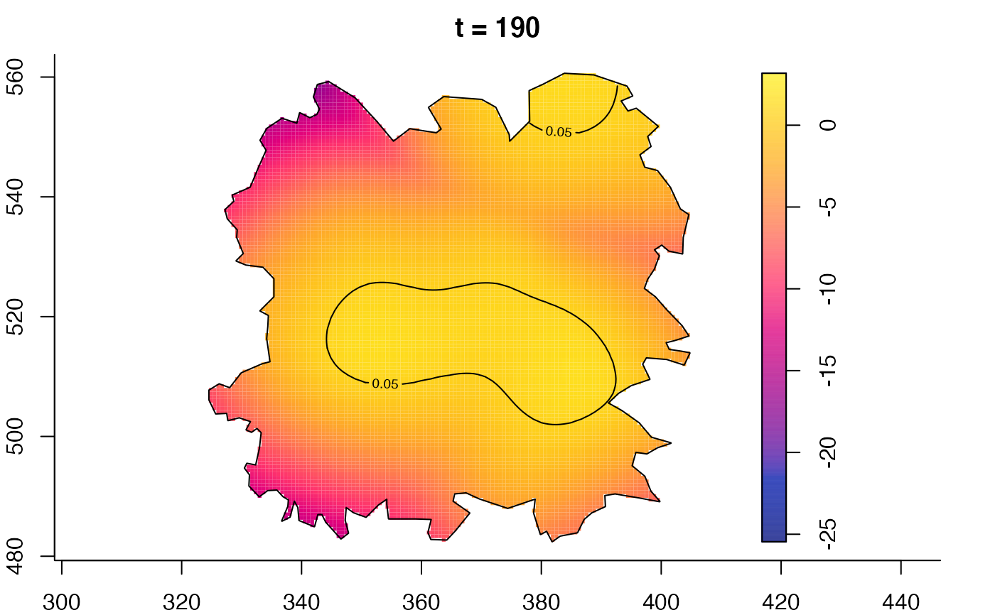
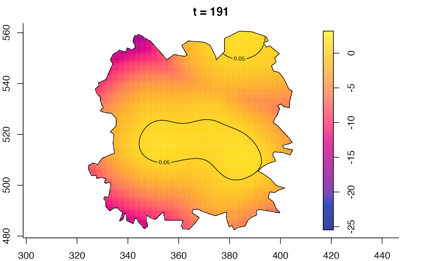
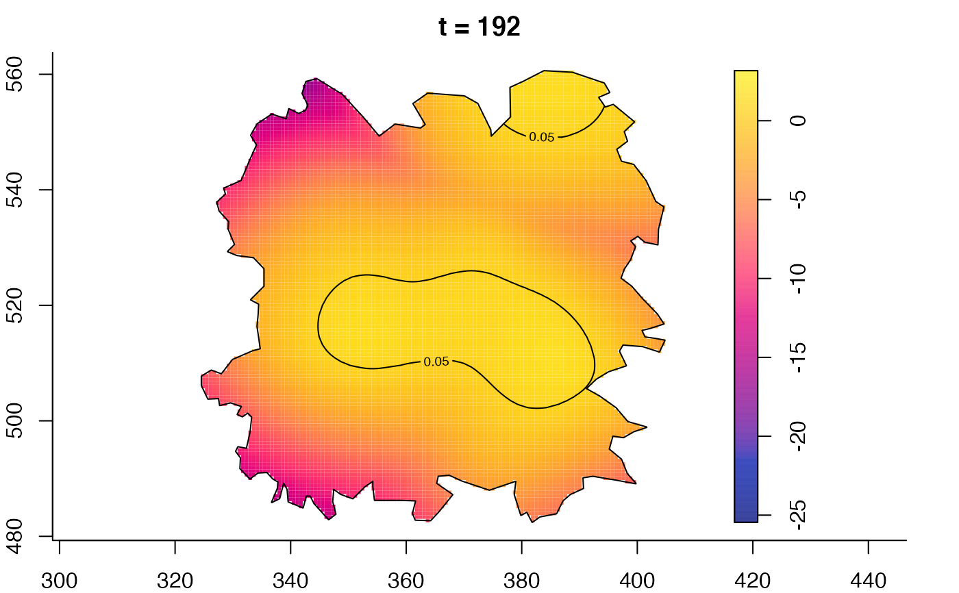


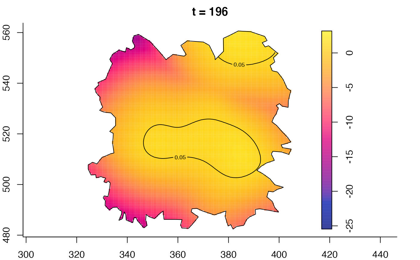
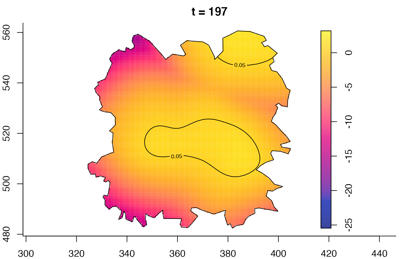


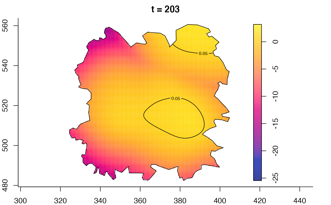


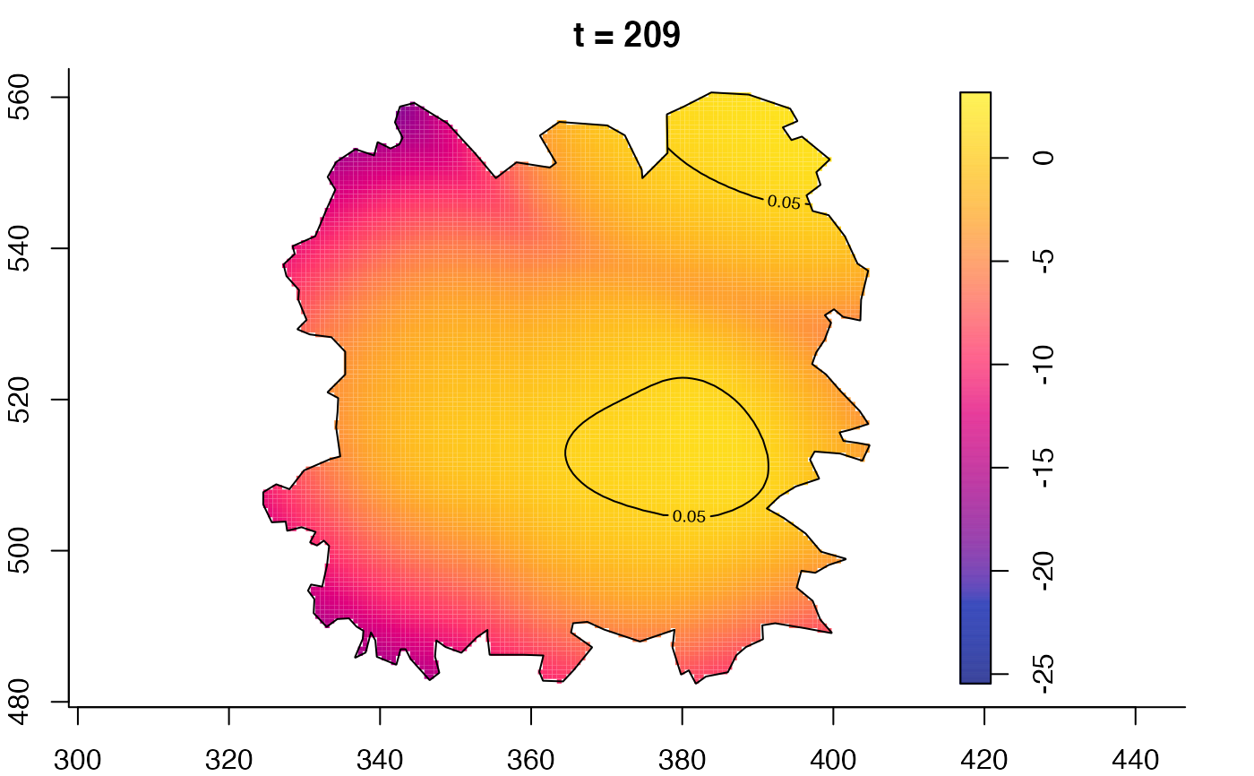
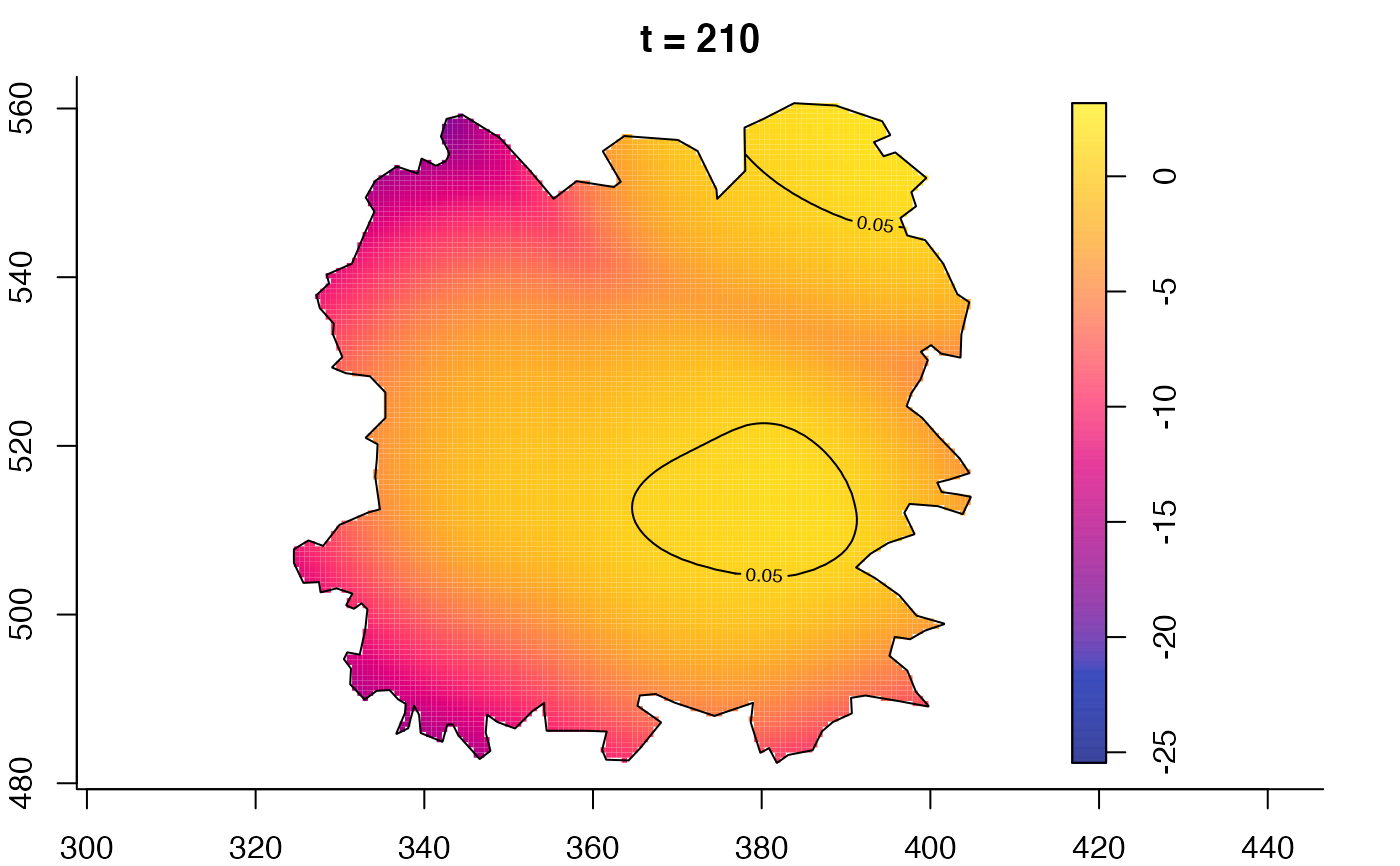
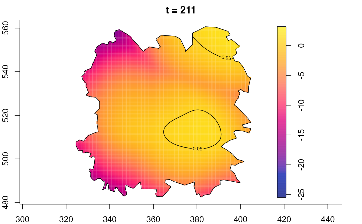
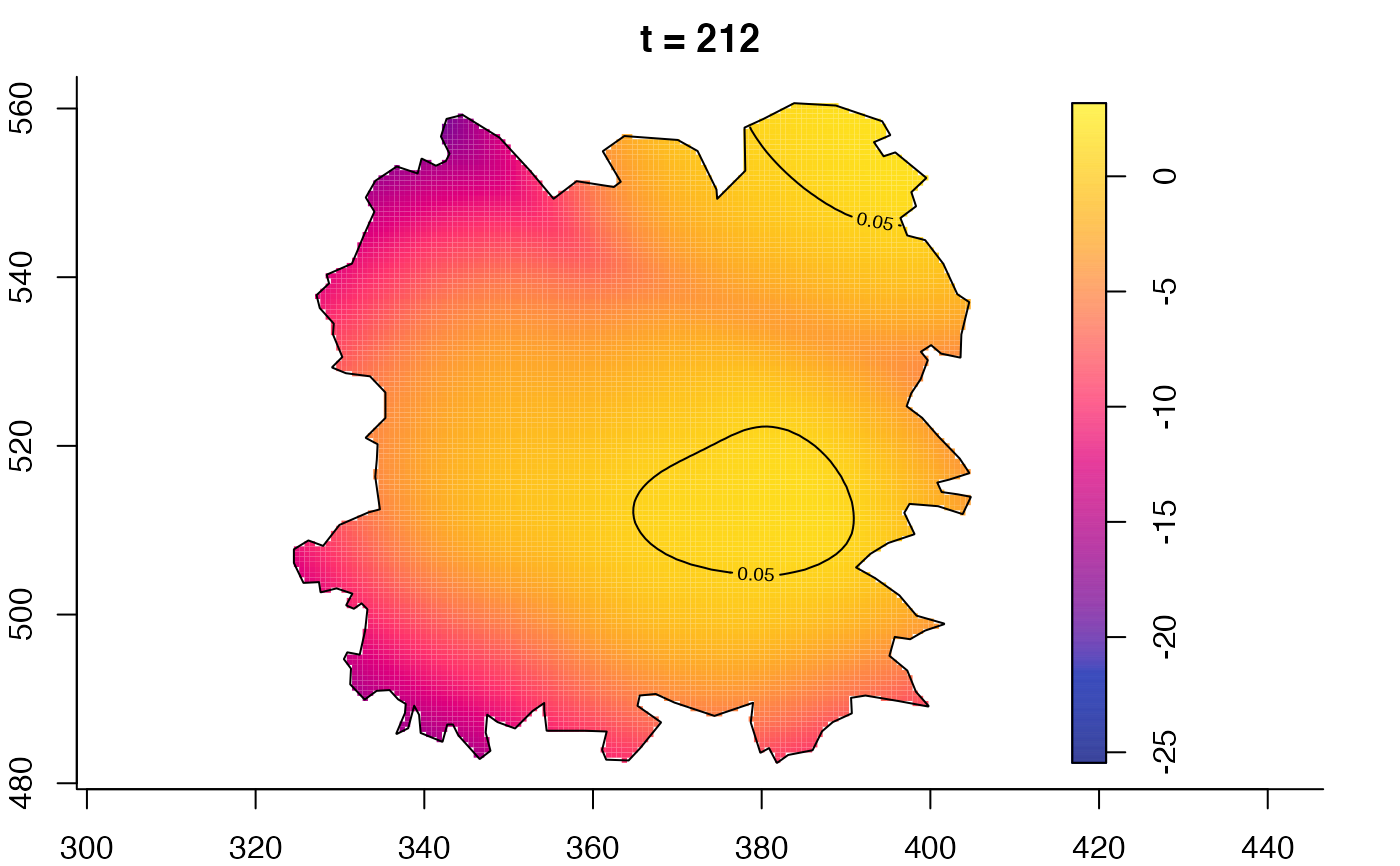
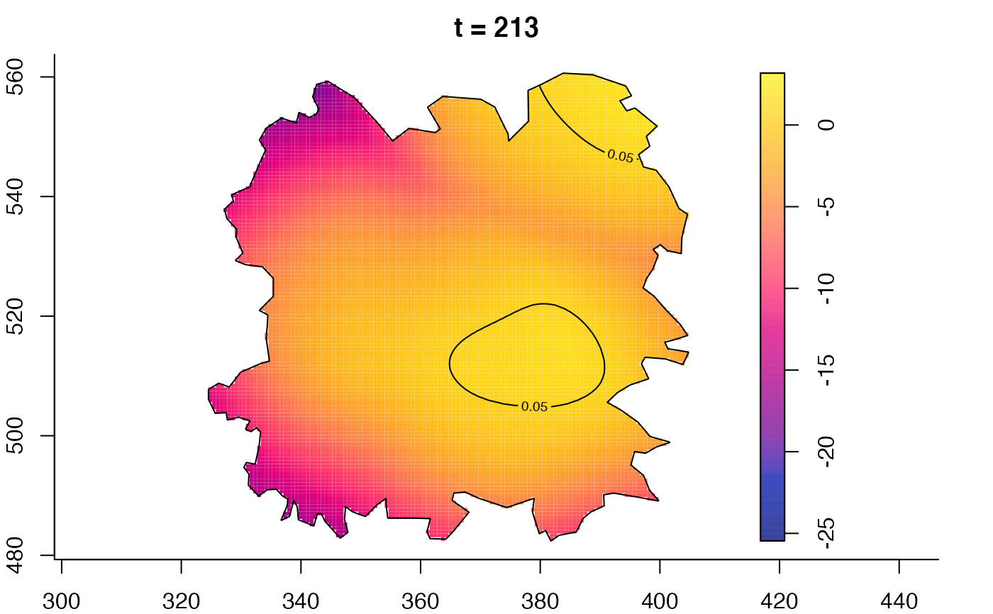
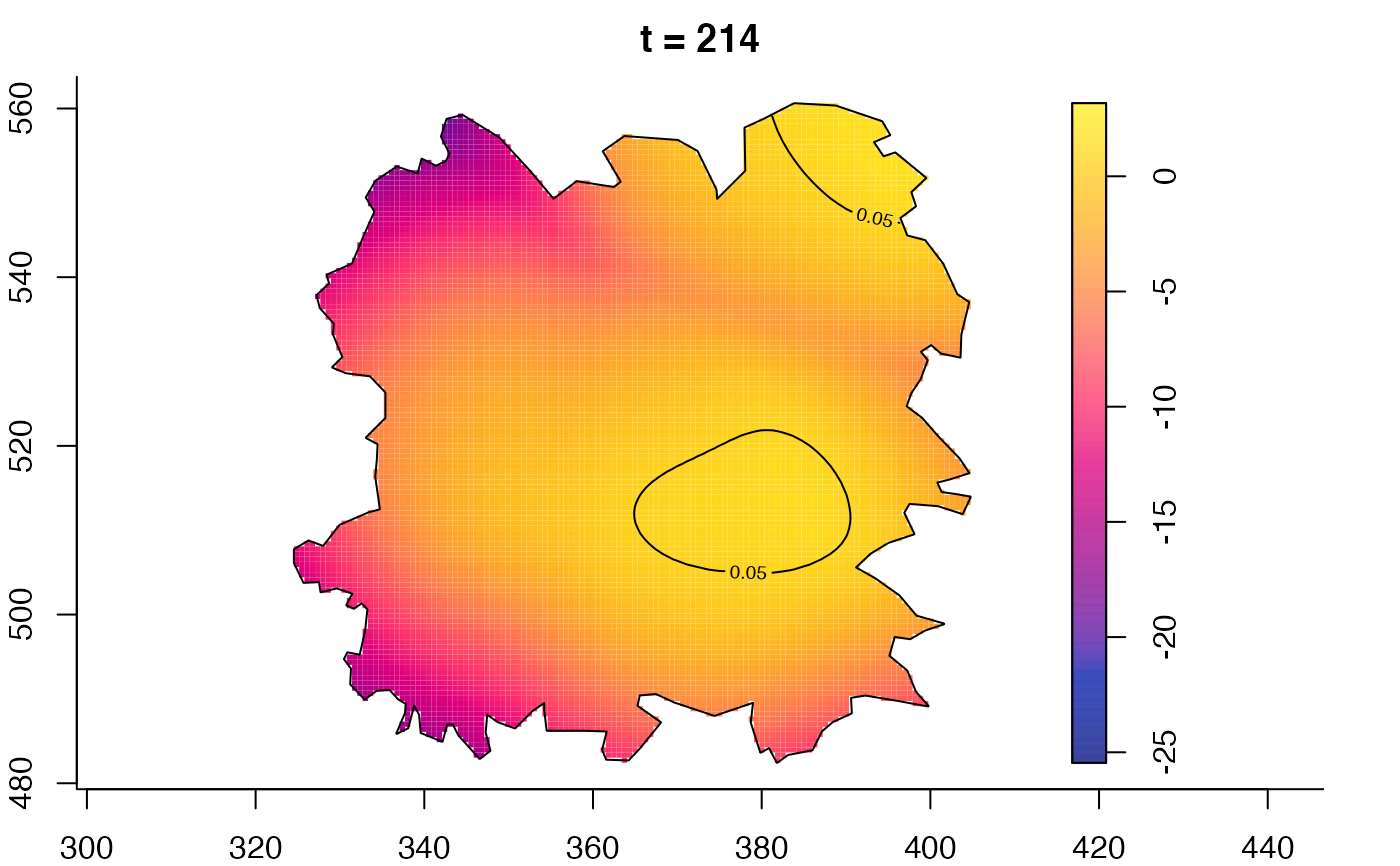


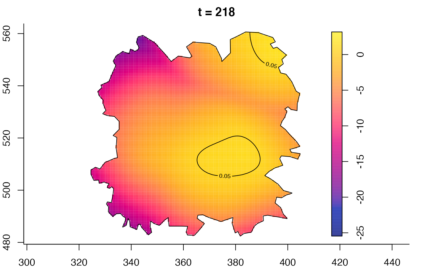

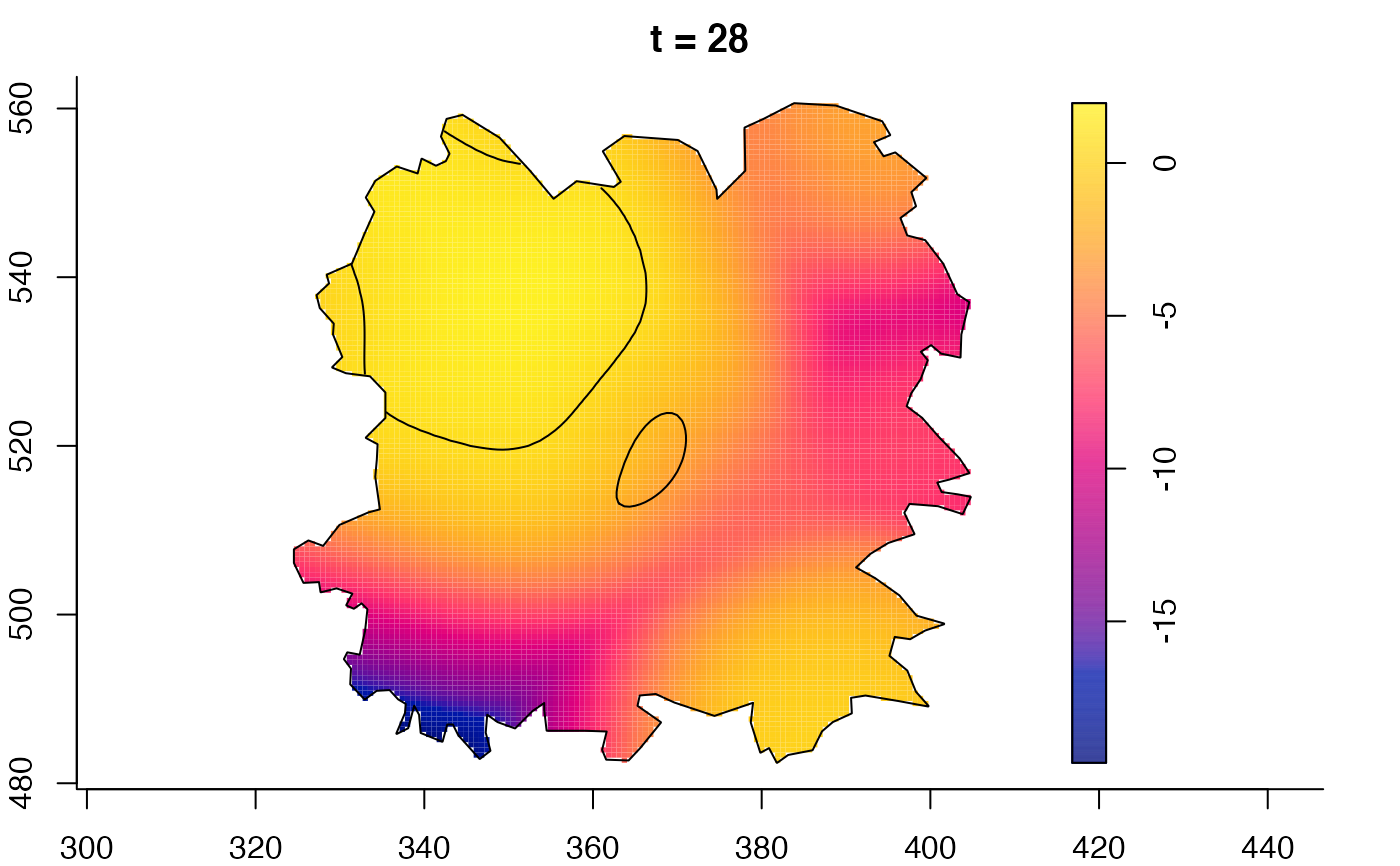
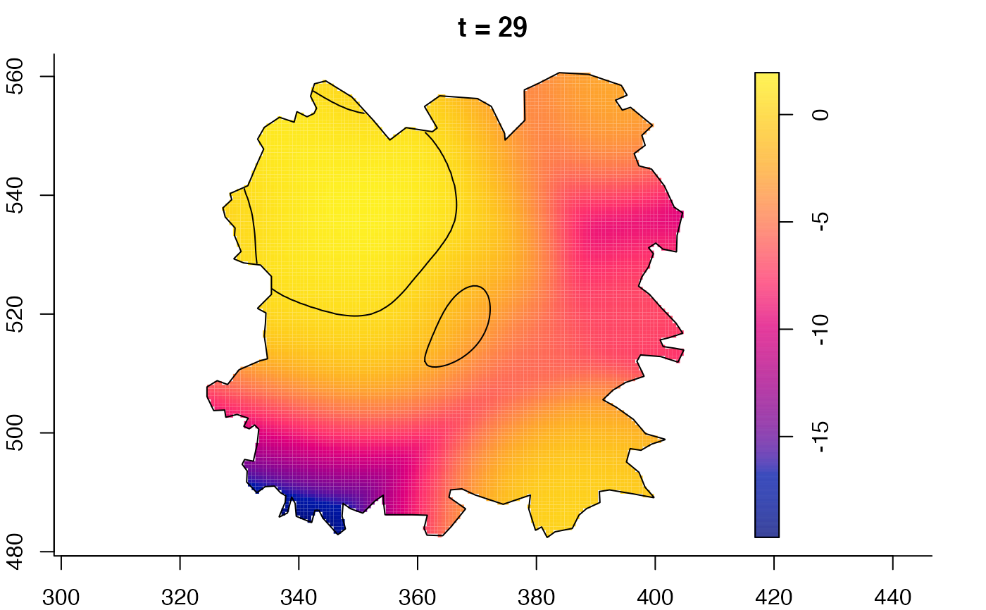
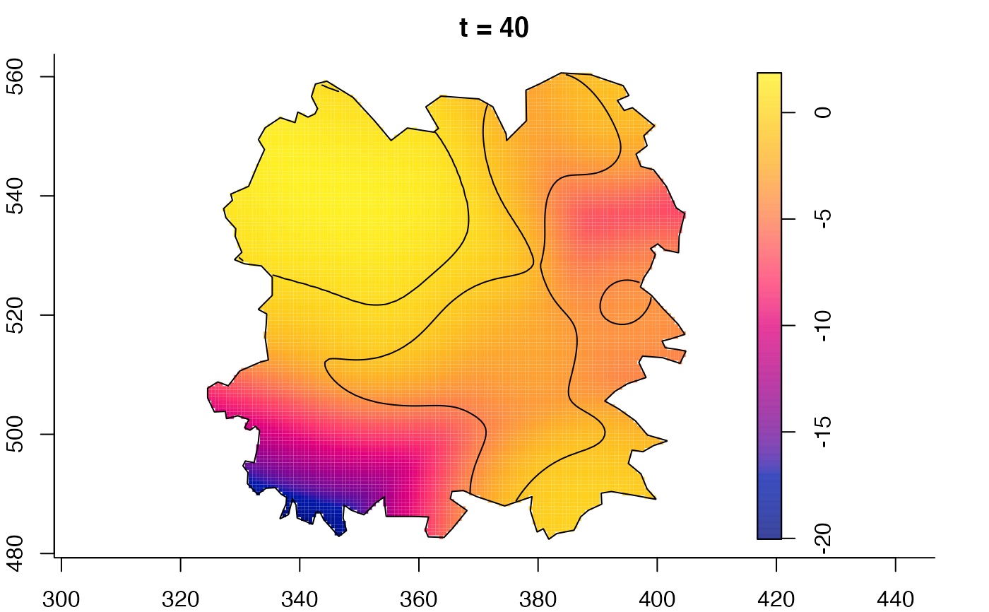
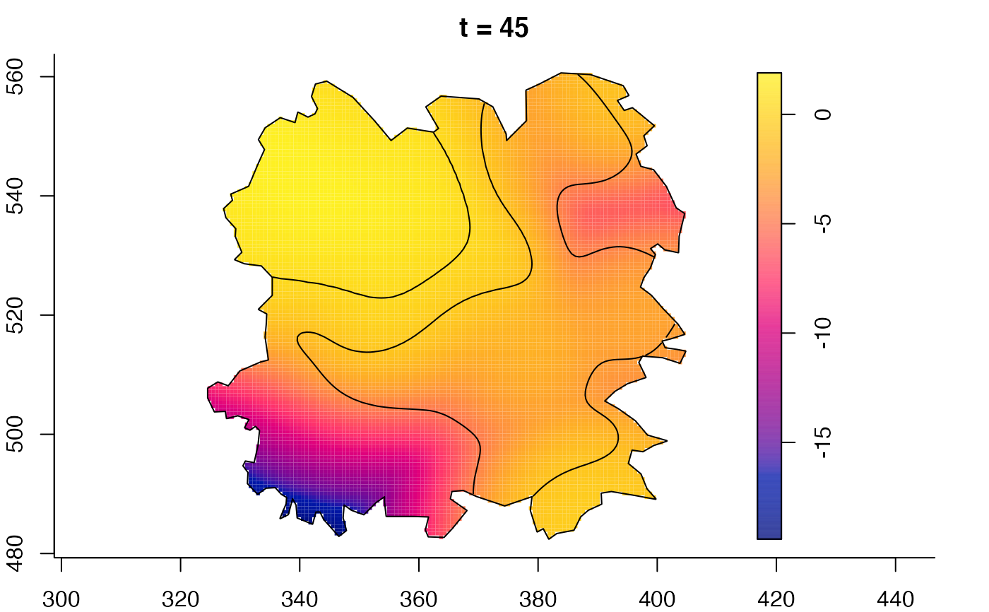
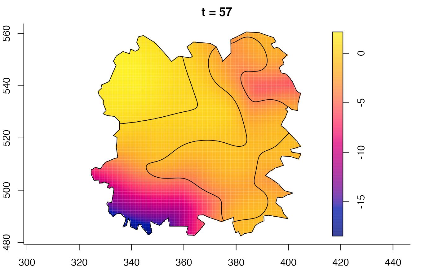
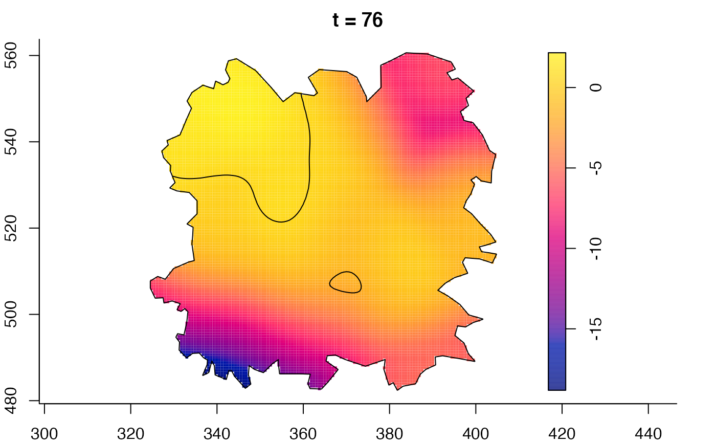
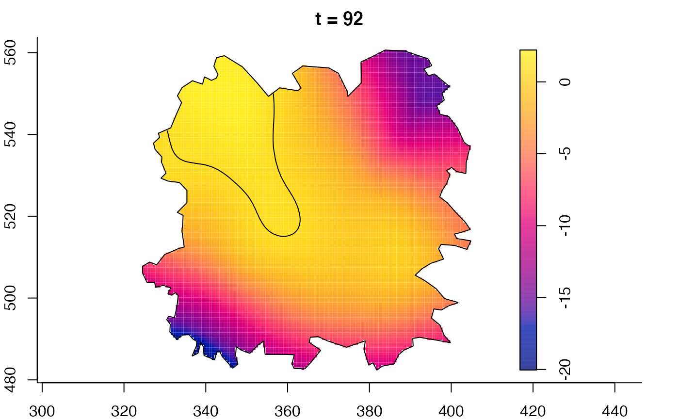
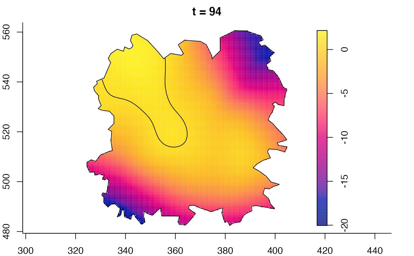
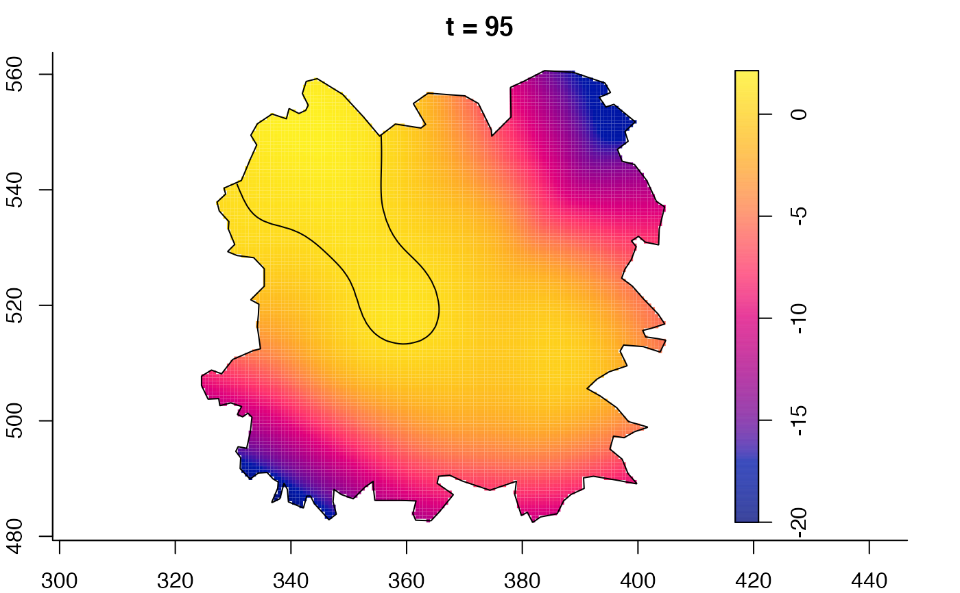
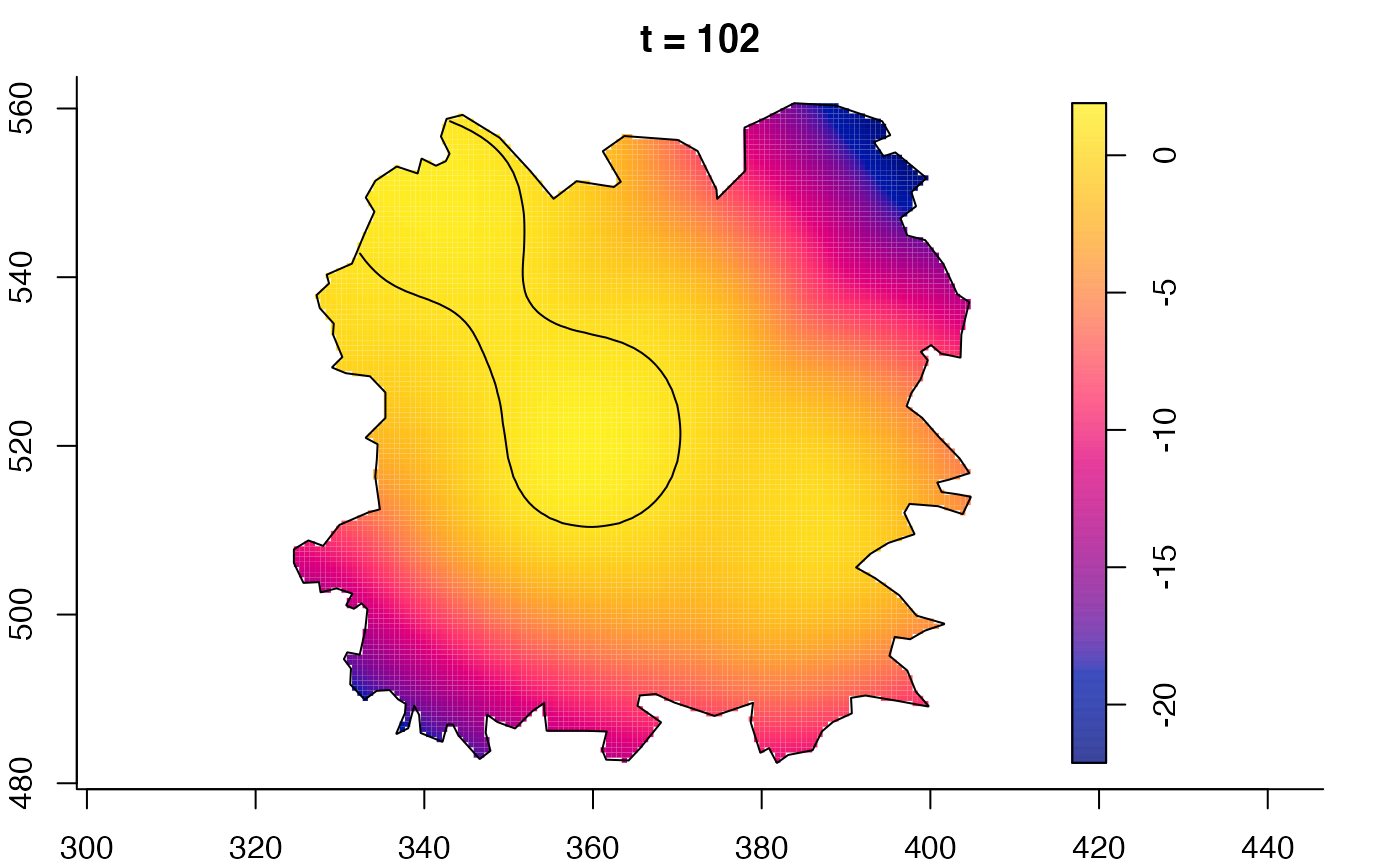
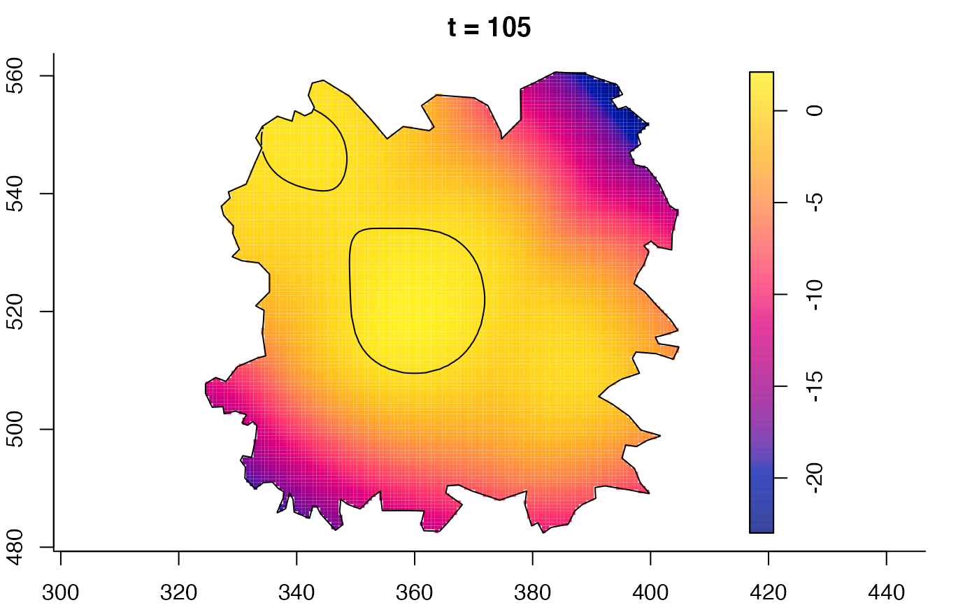
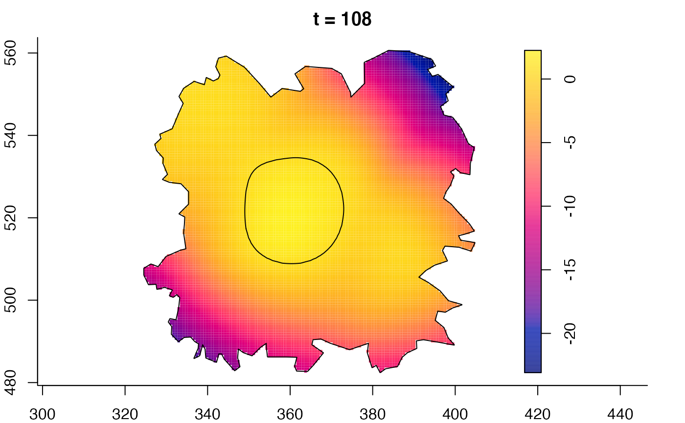
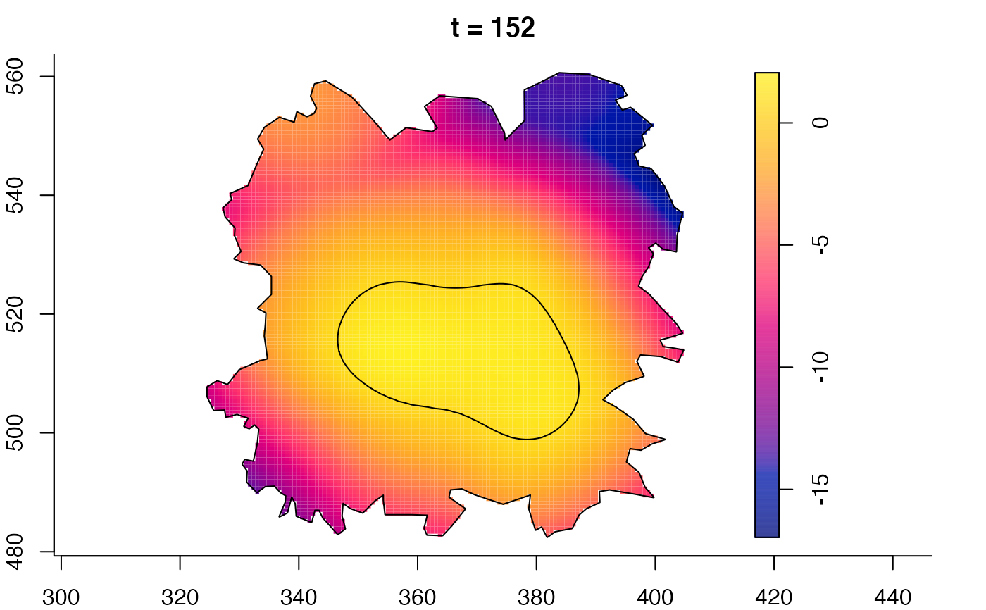
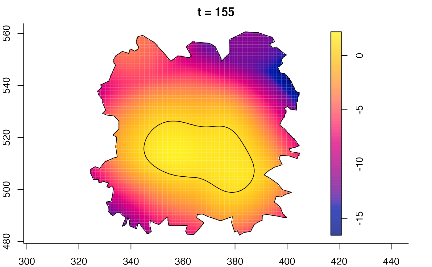
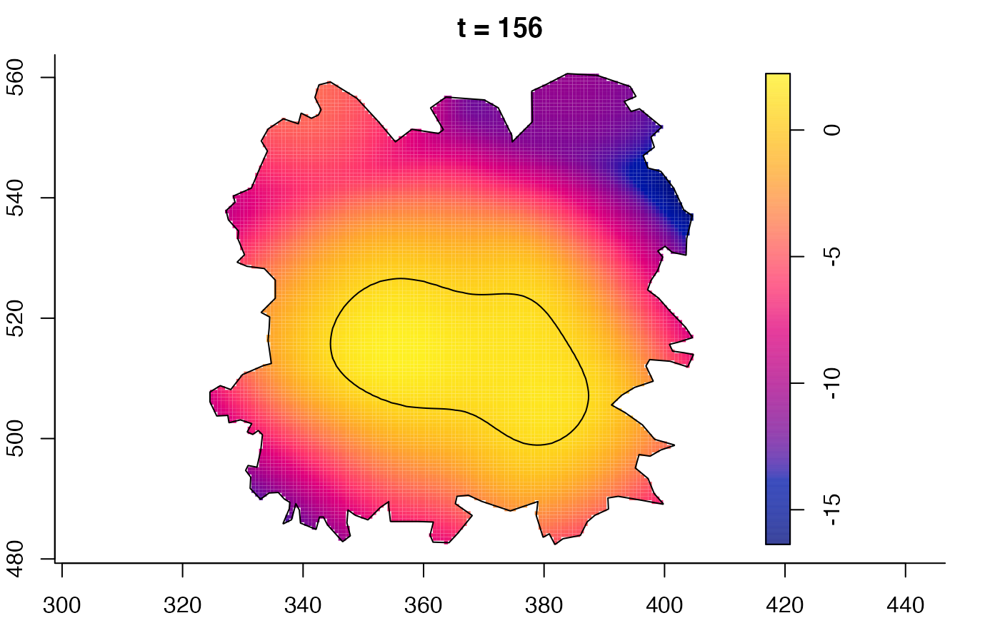
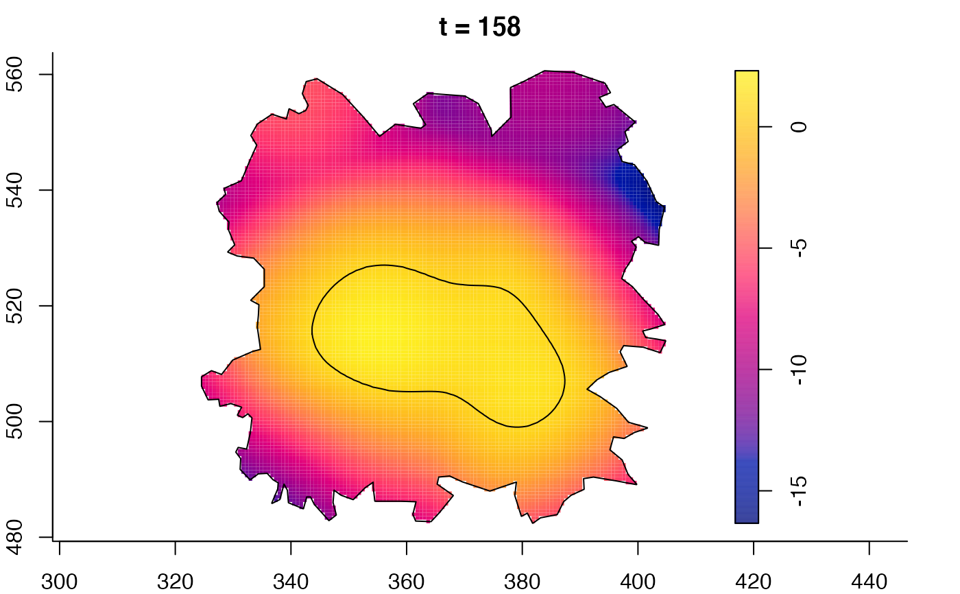
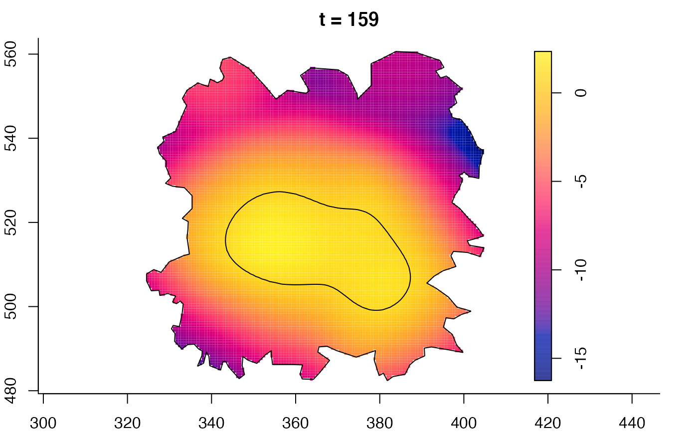
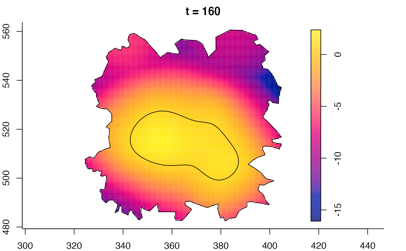
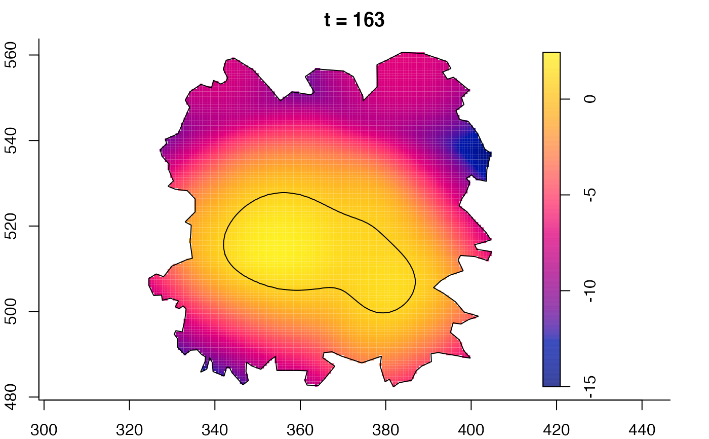
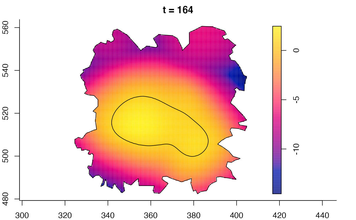
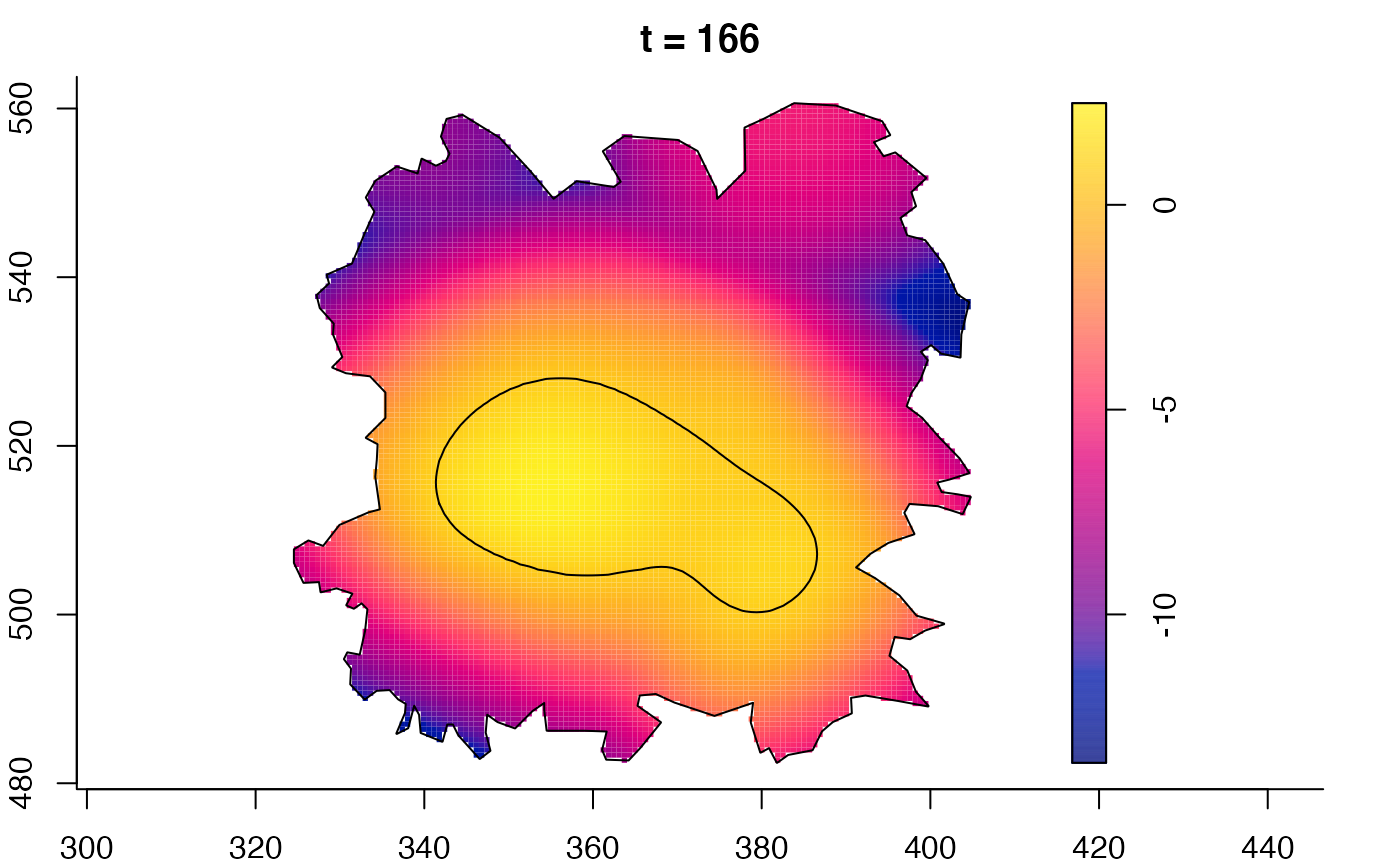
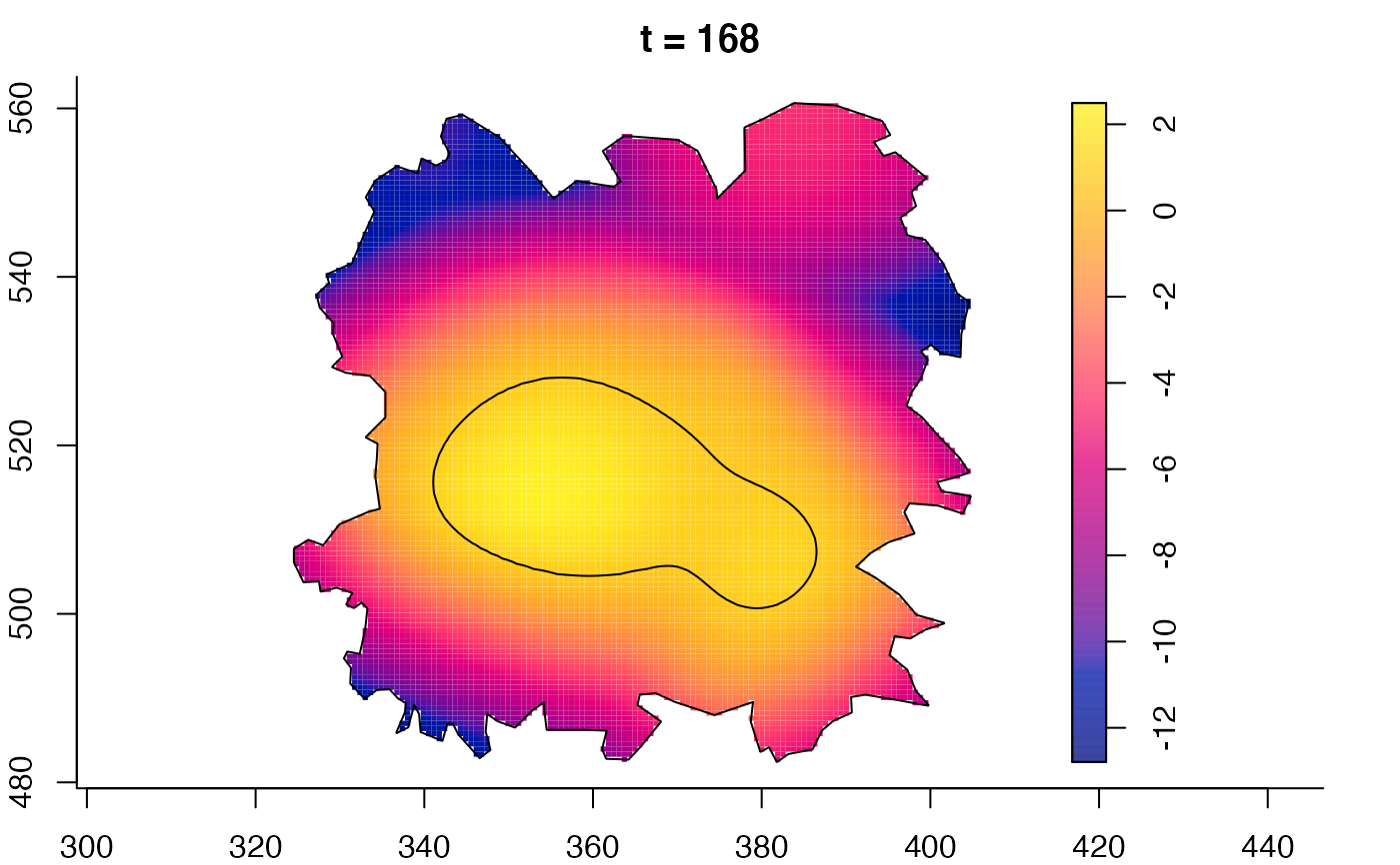
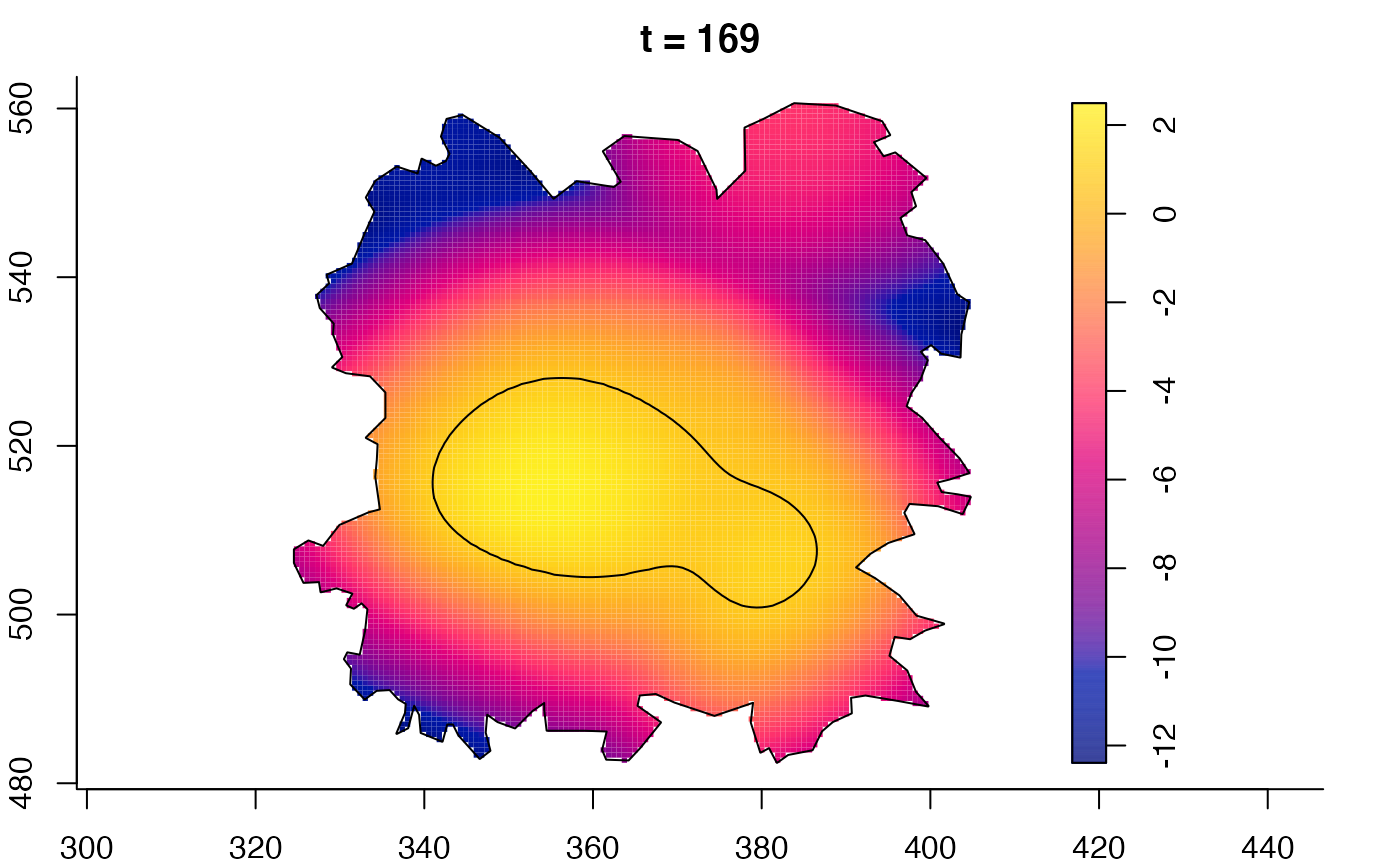
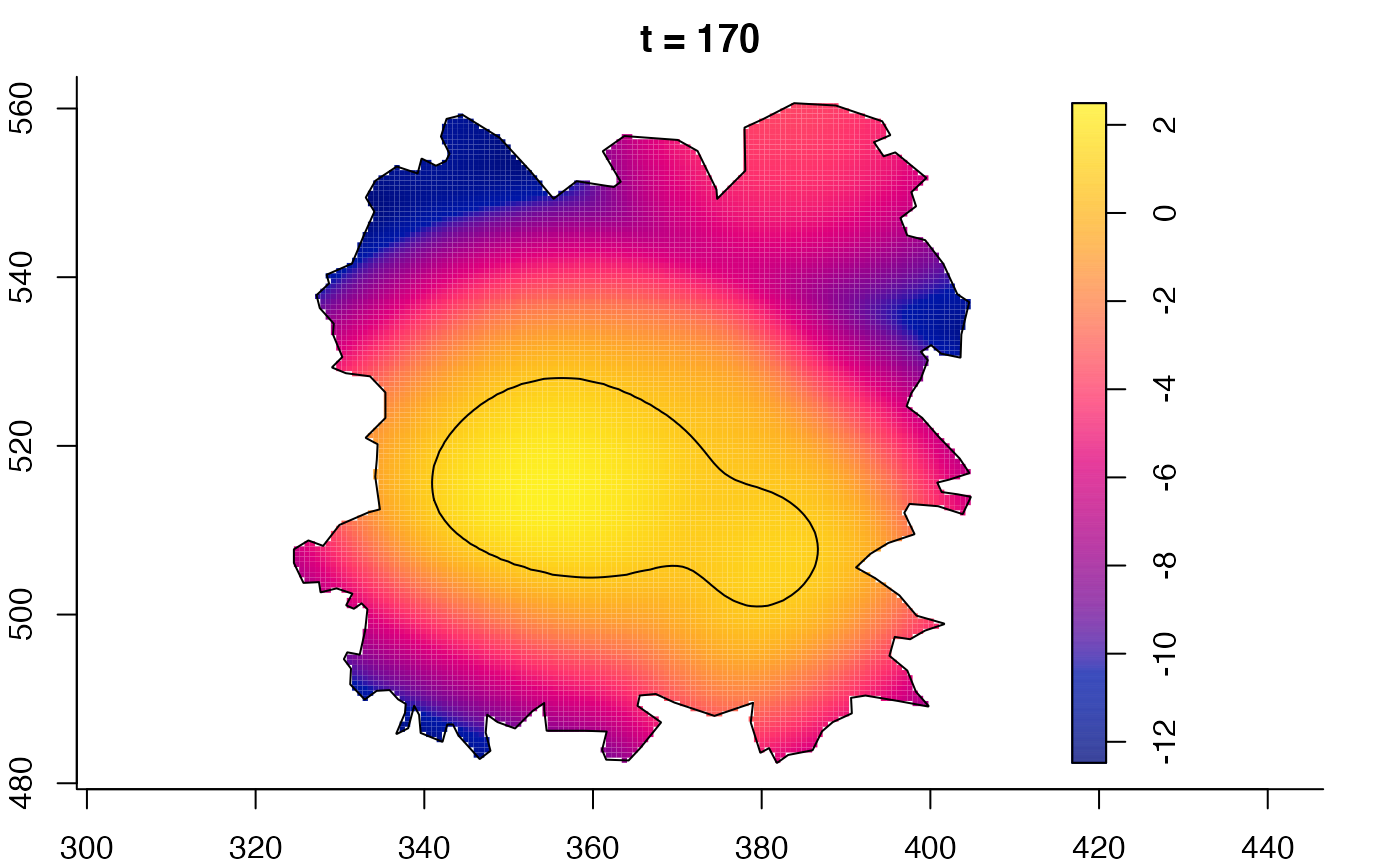
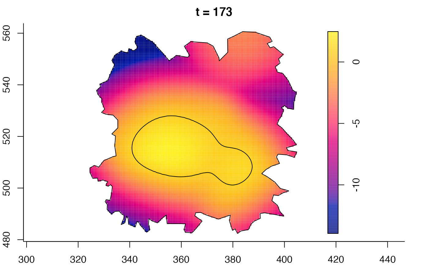
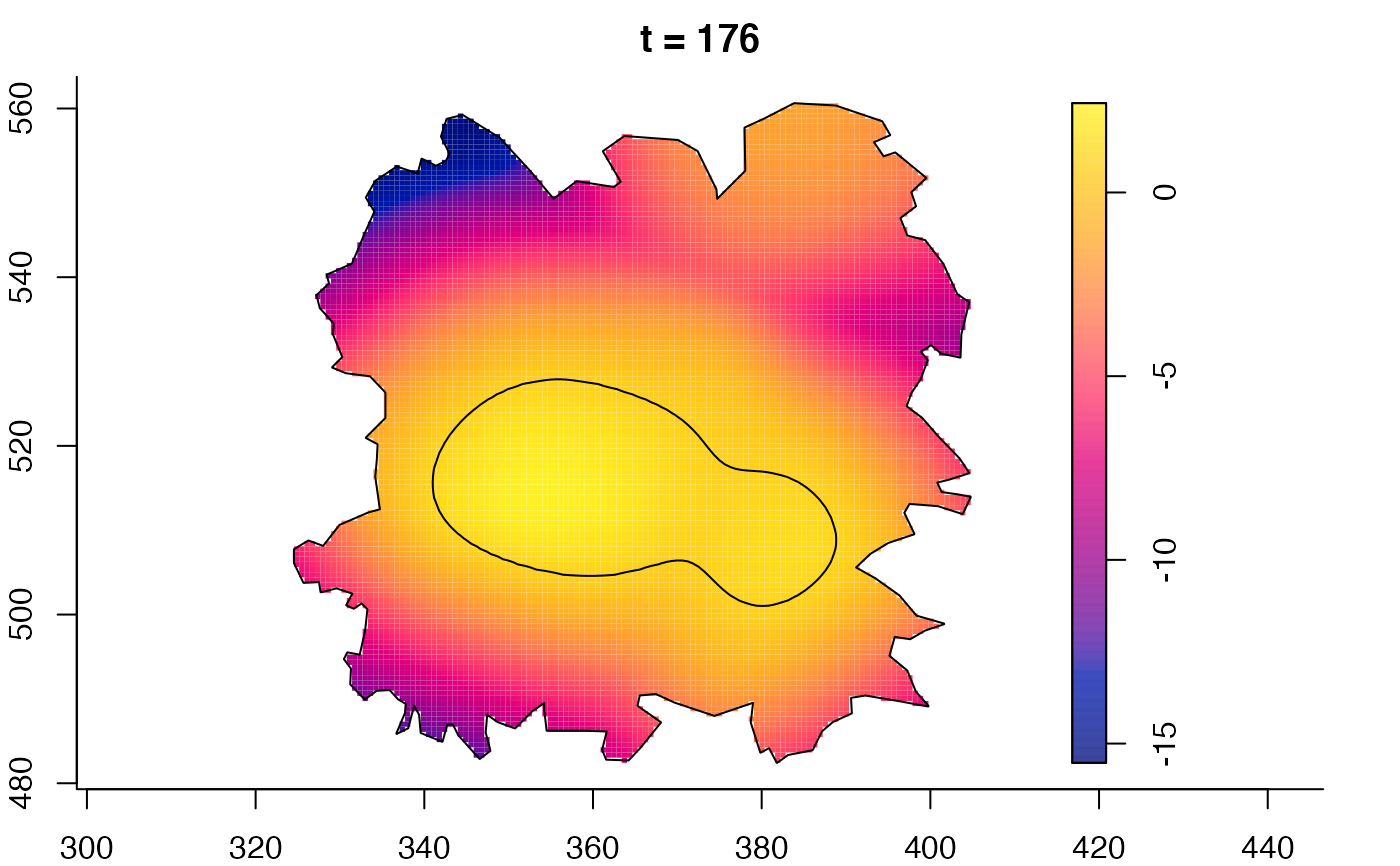
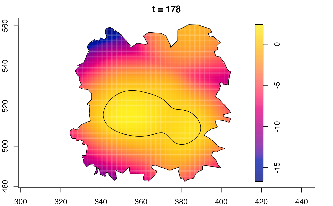
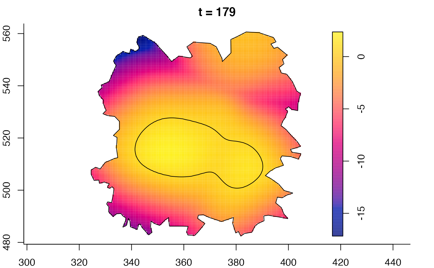
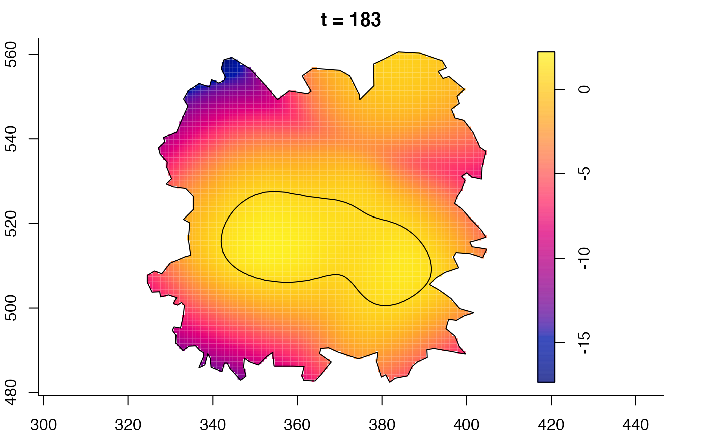
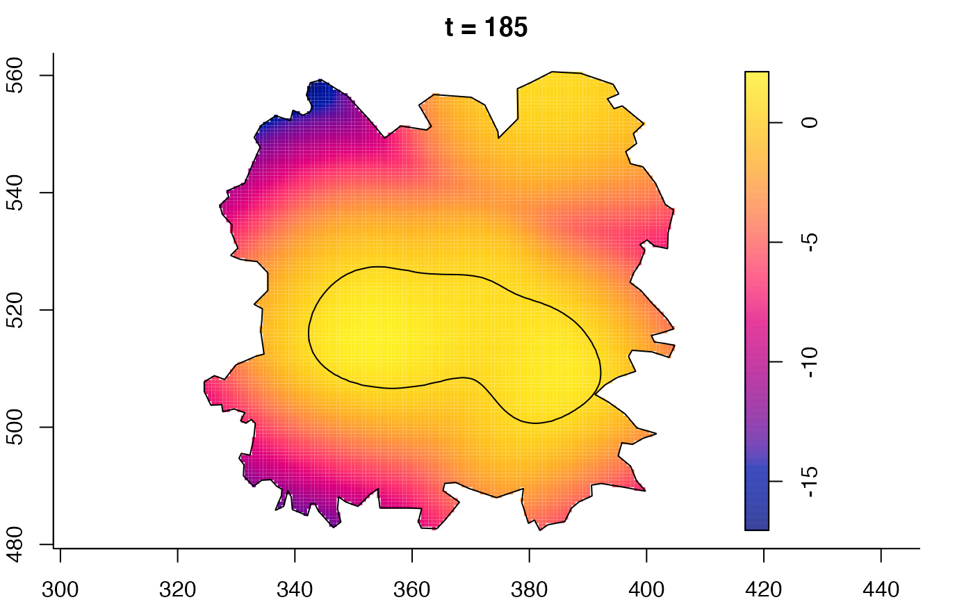
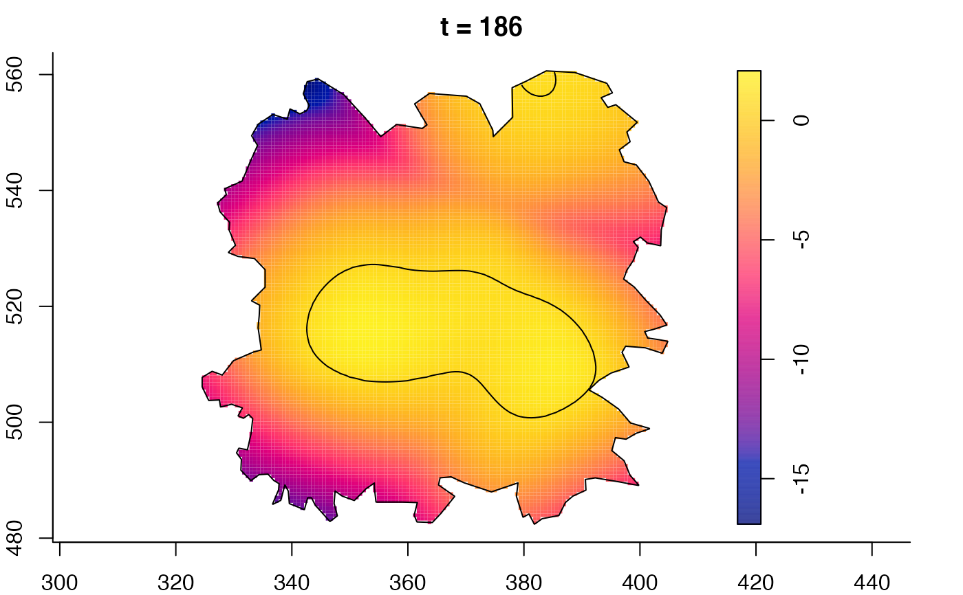
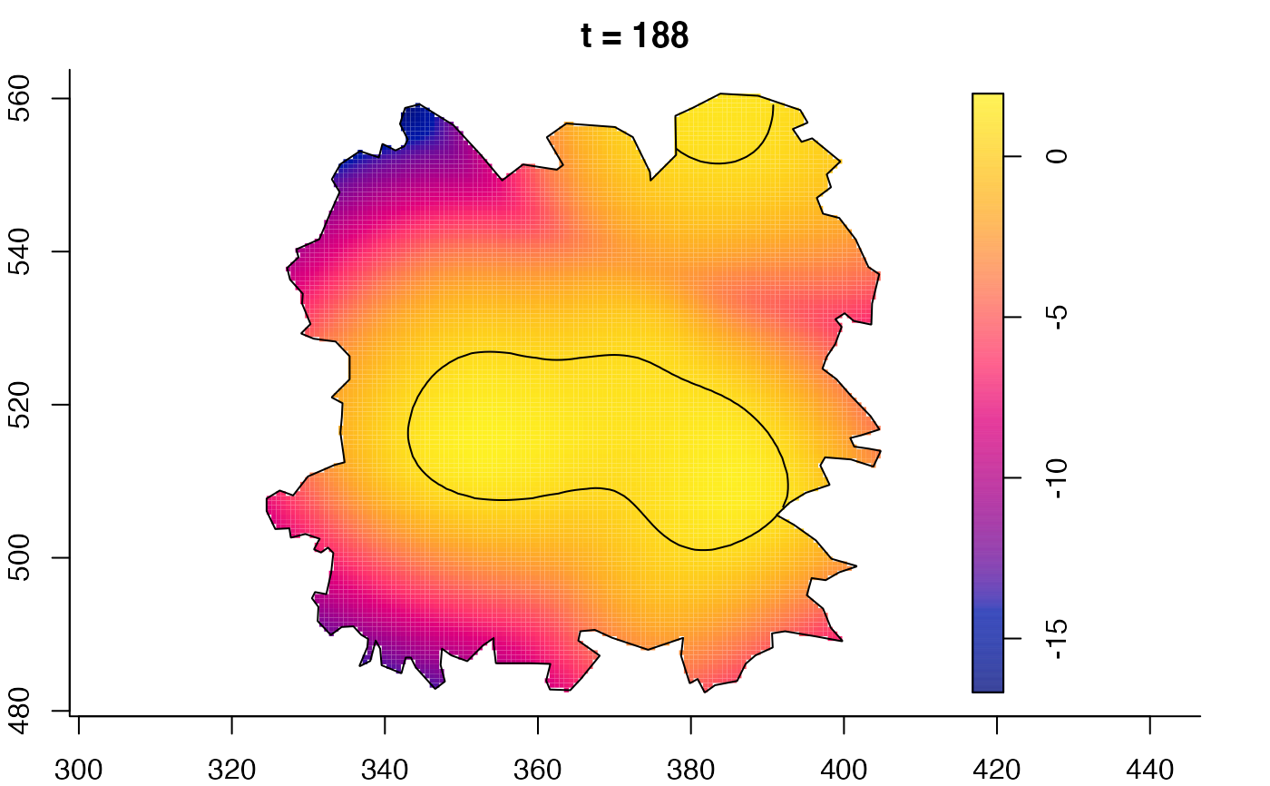
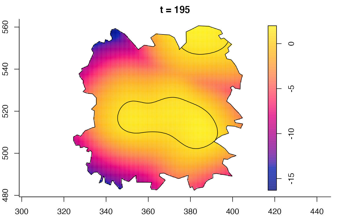
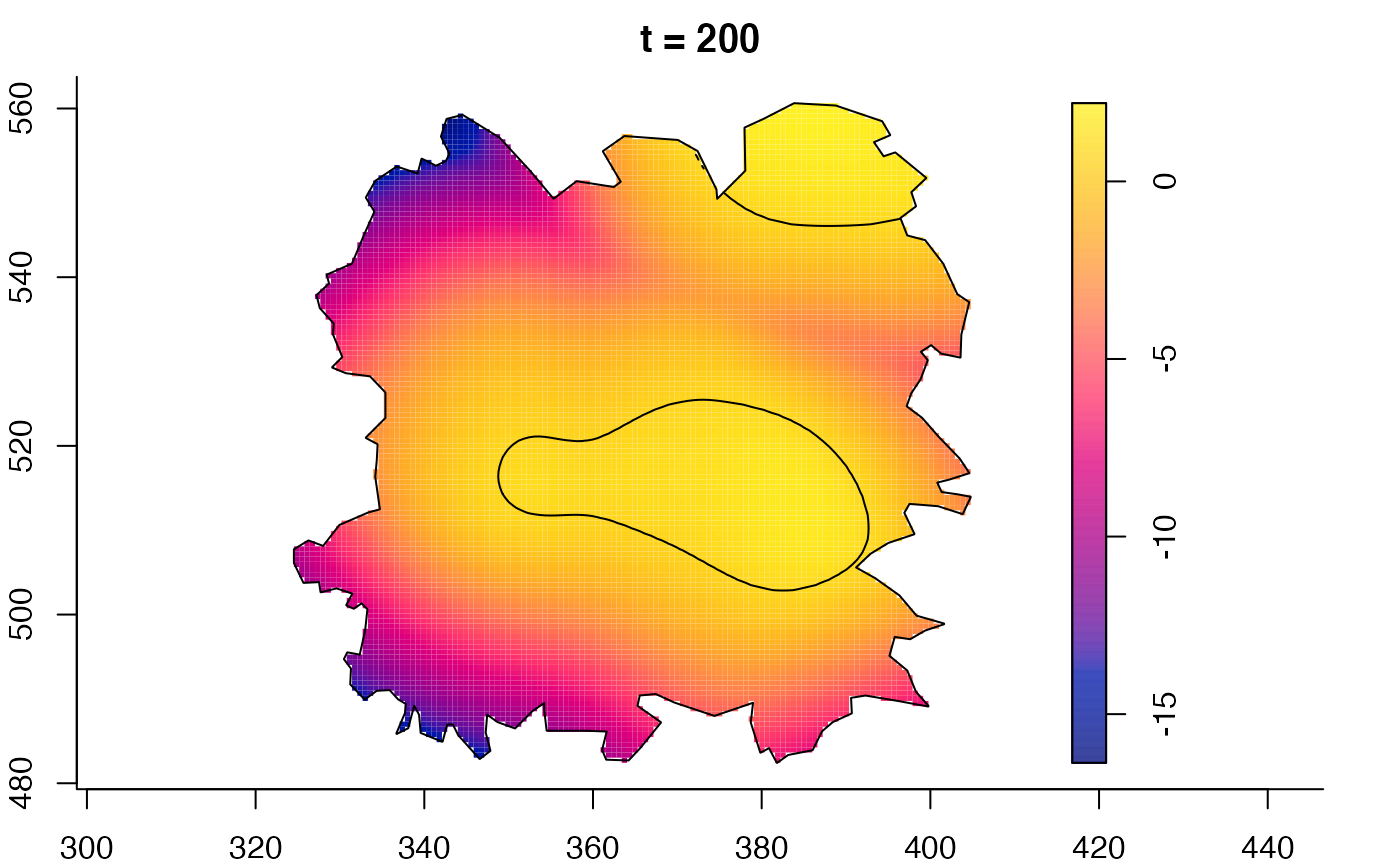
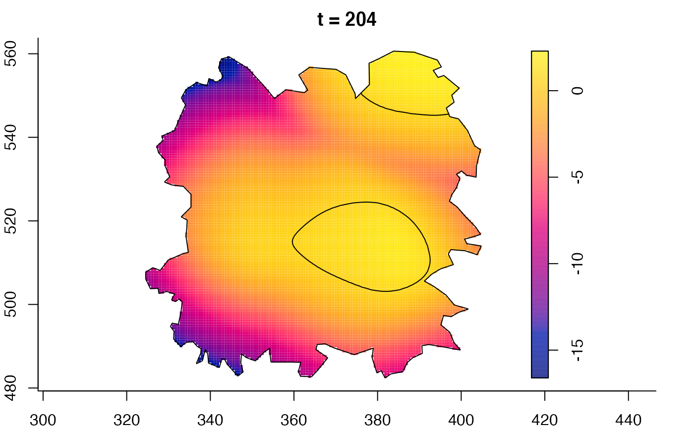
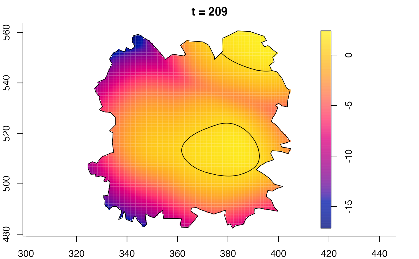
 plot(fmdrr,type="conditional",sleep=0.1,tol.type="two.sided",
tol.args=list(levels=0.05,drawlabels=FALSE))
plot(fmdrr,type="conditional",sleep=0.1,tol.type="two.sided",
tol.args=list(levels=0.05,drawlabels=FALSE))


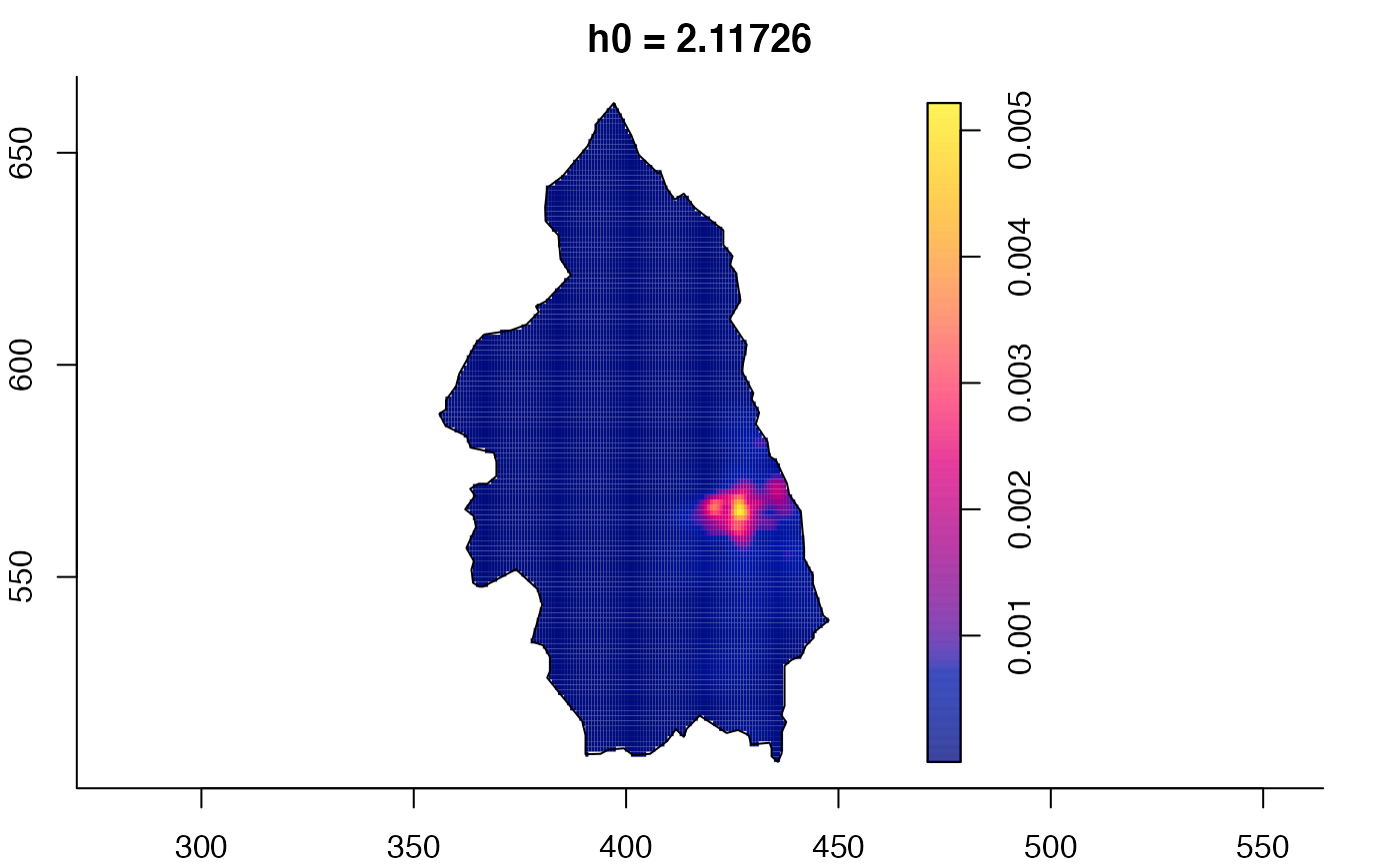
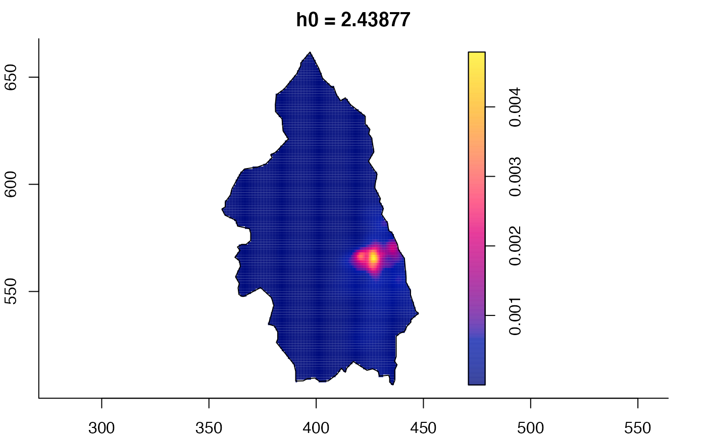
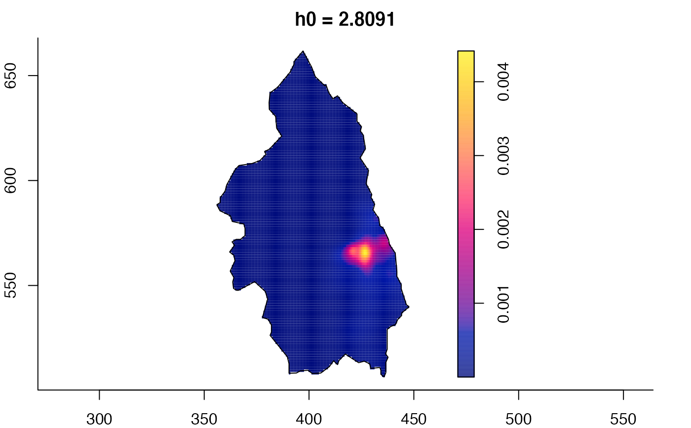
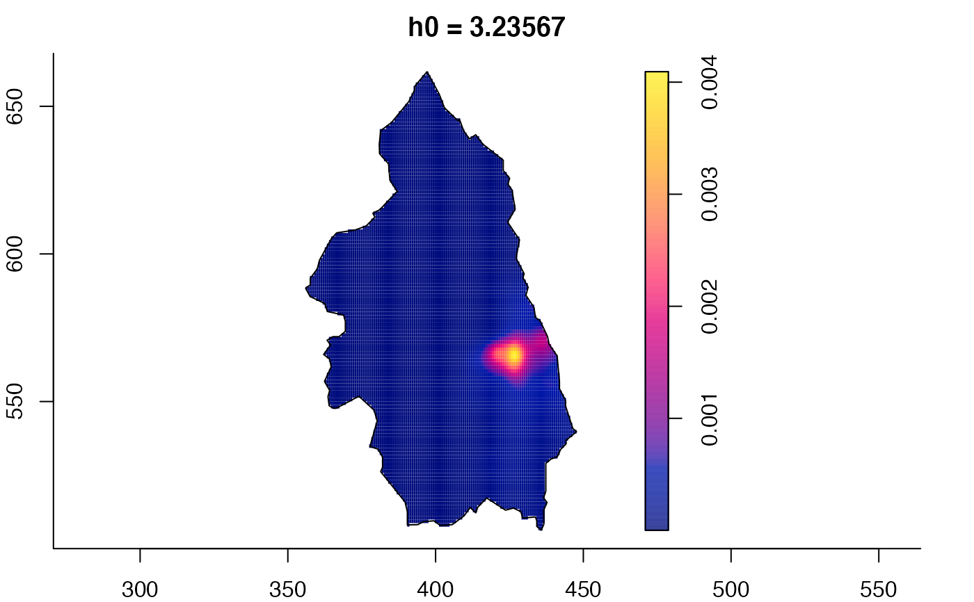
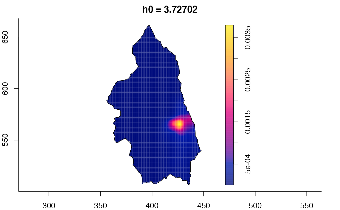
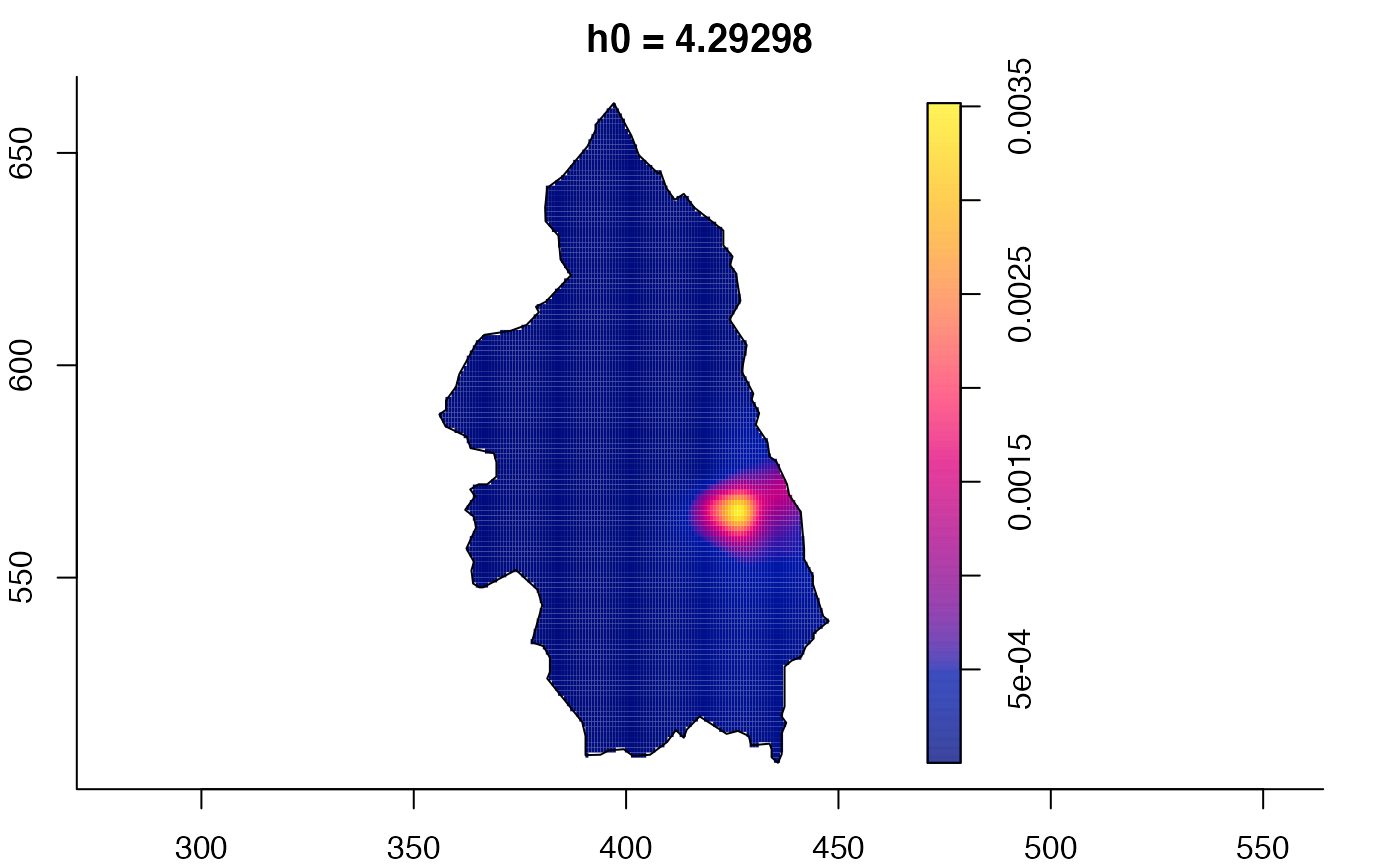
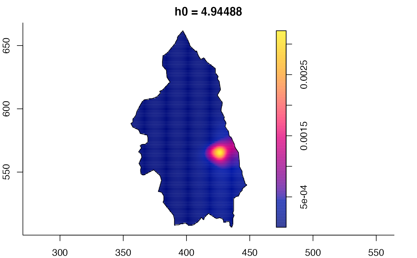
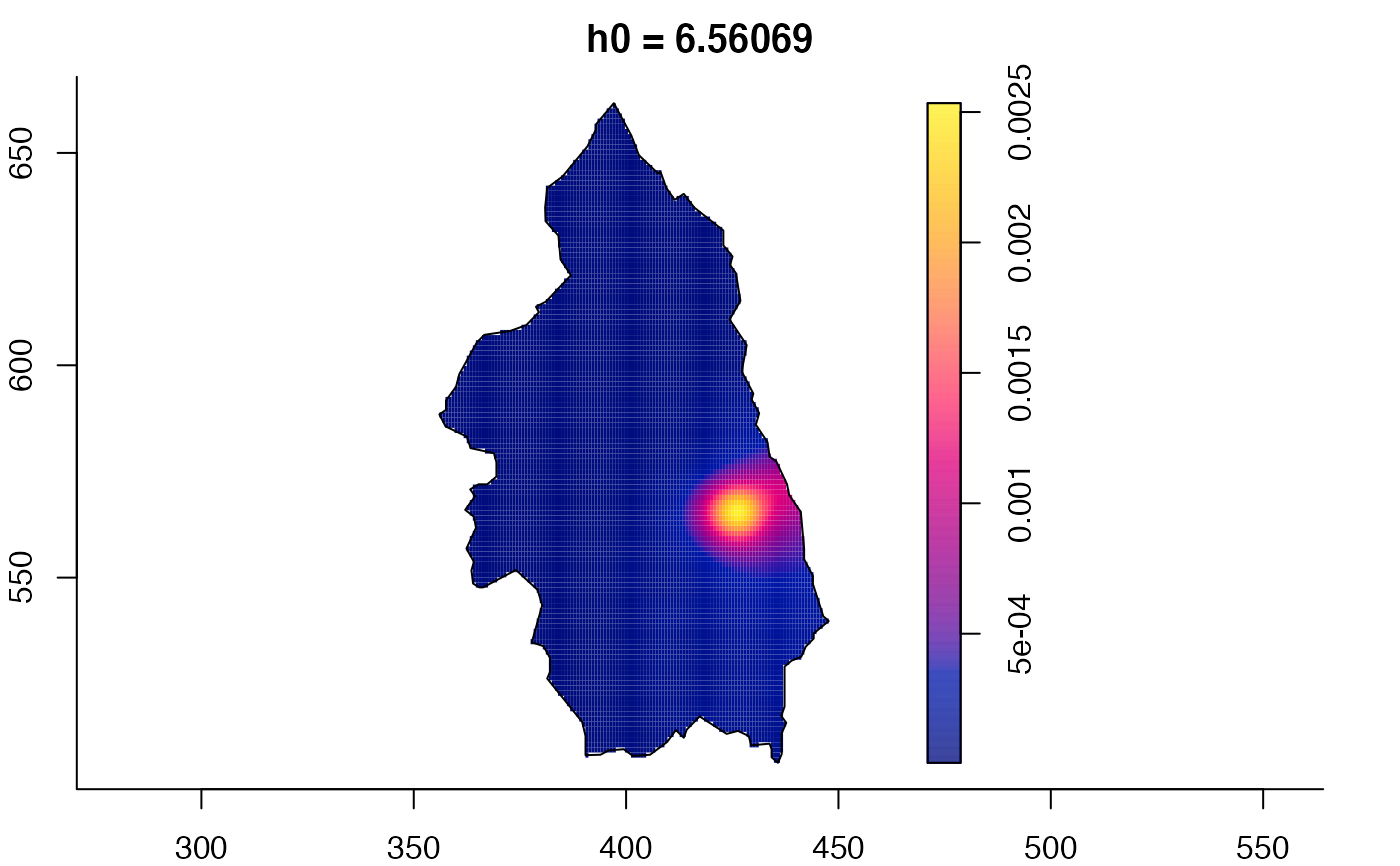
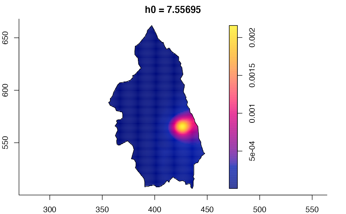
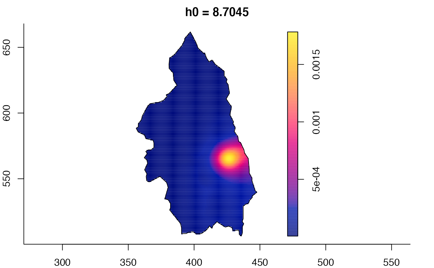
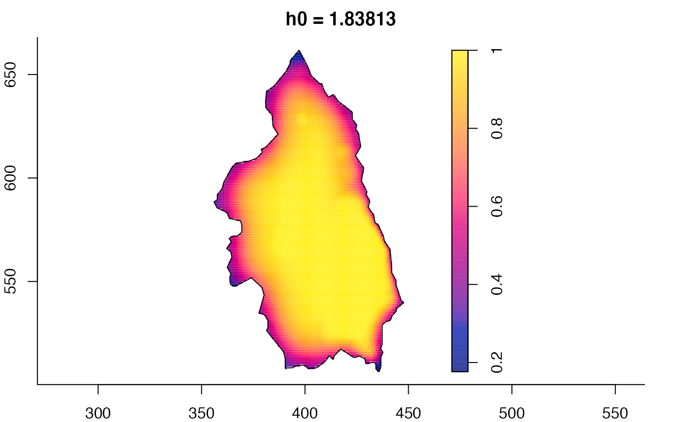
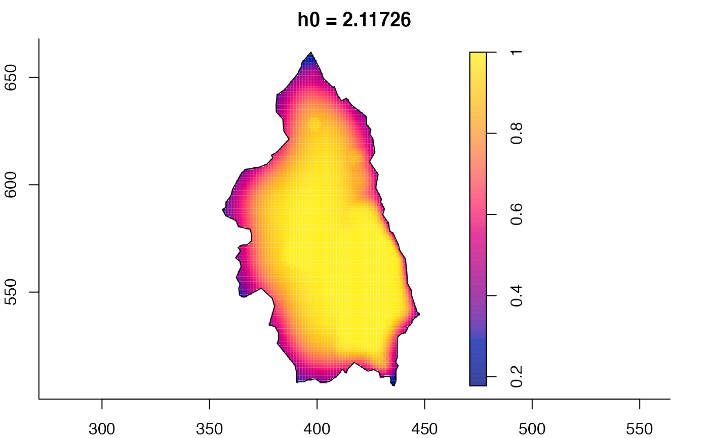
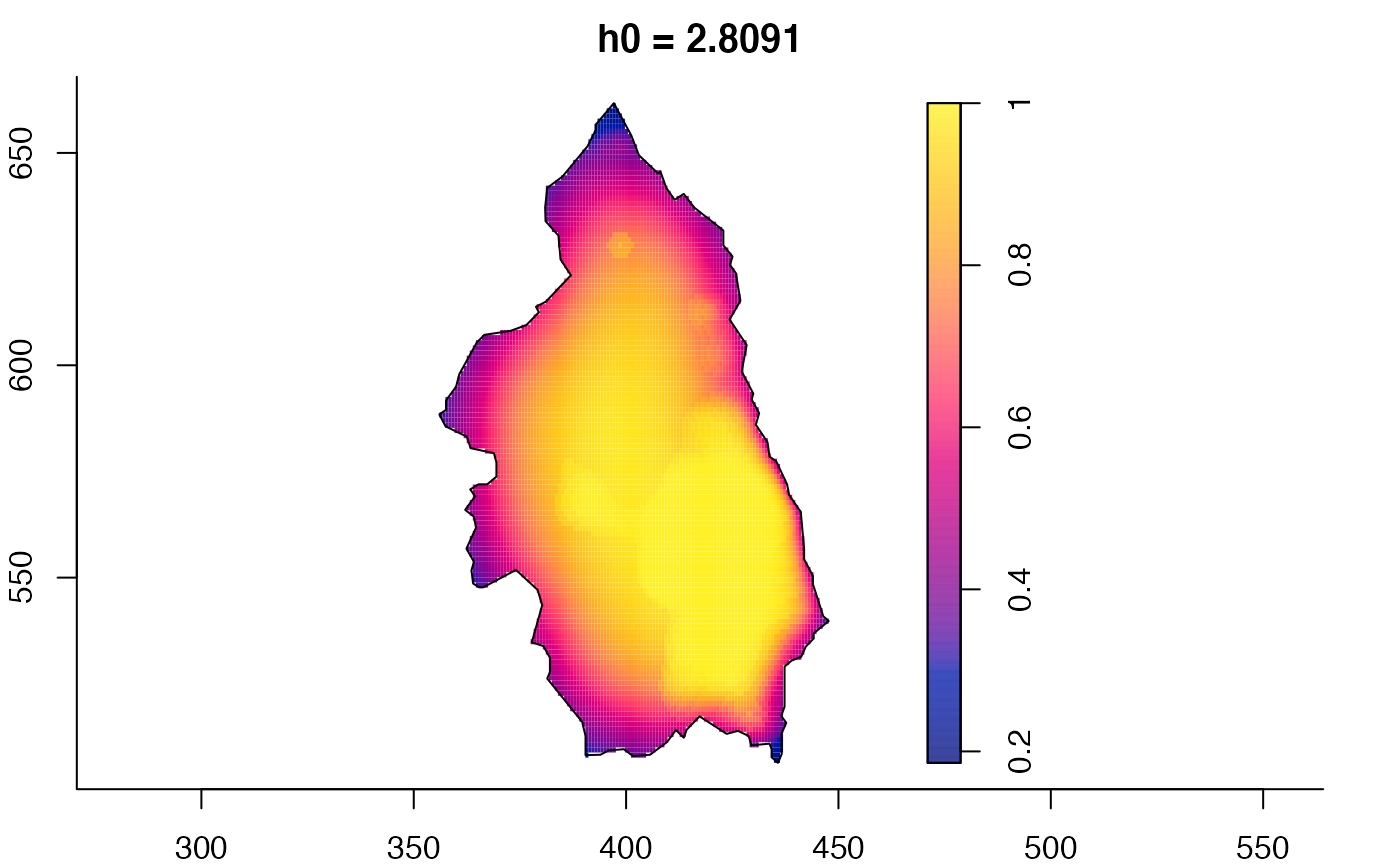
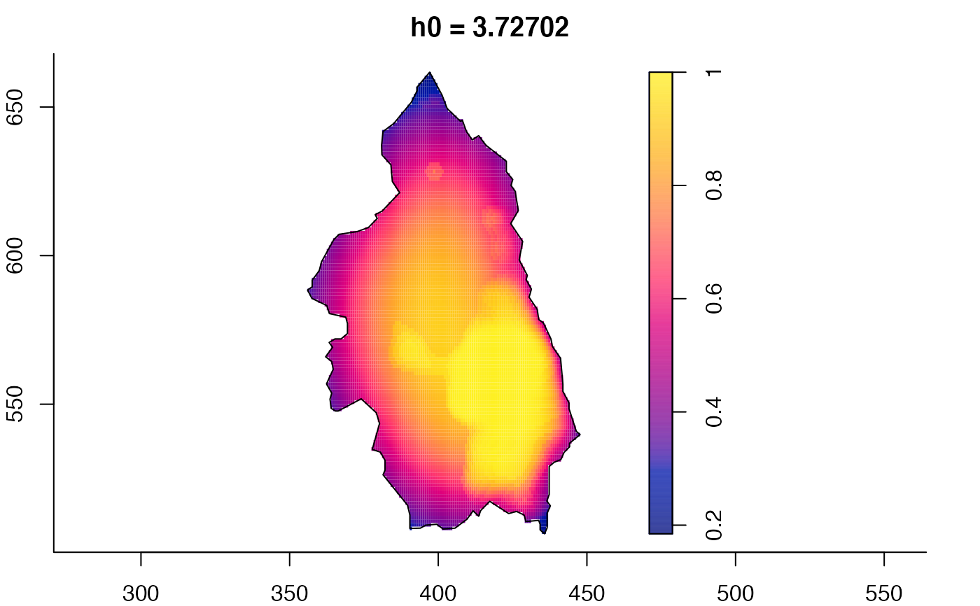
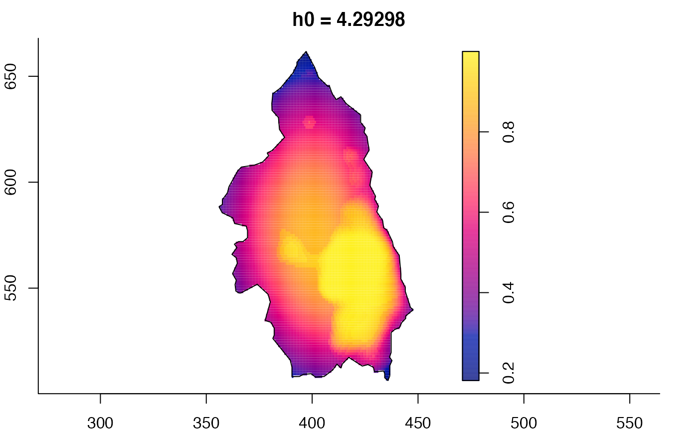
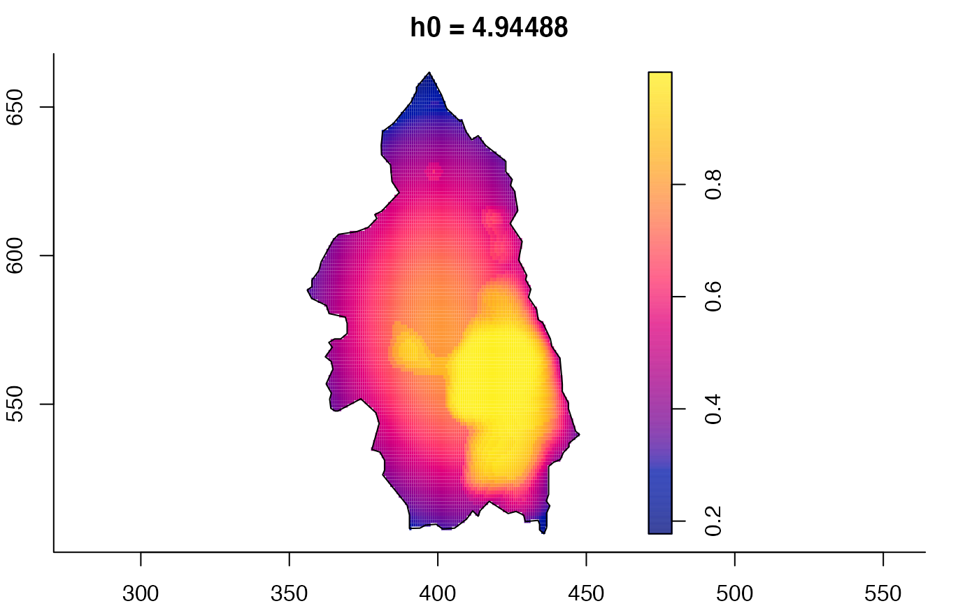
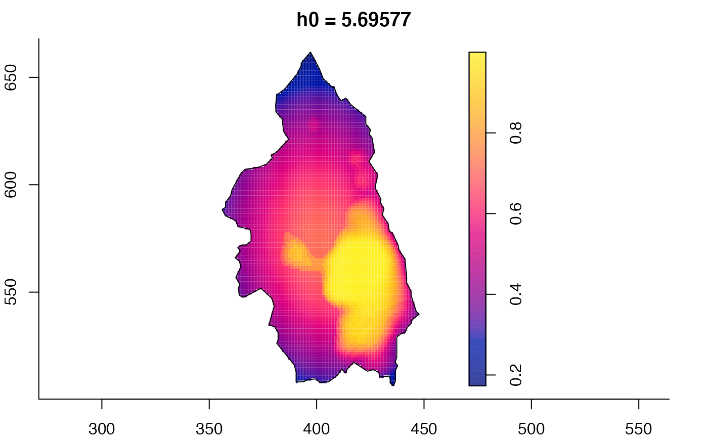
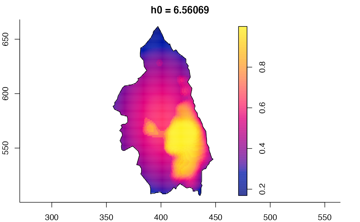
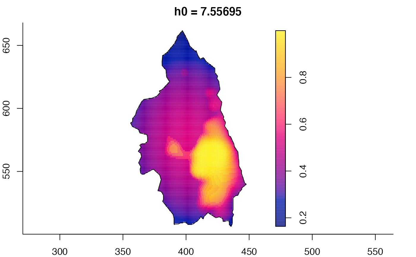
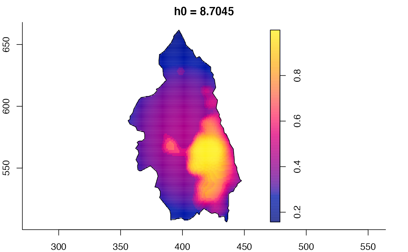
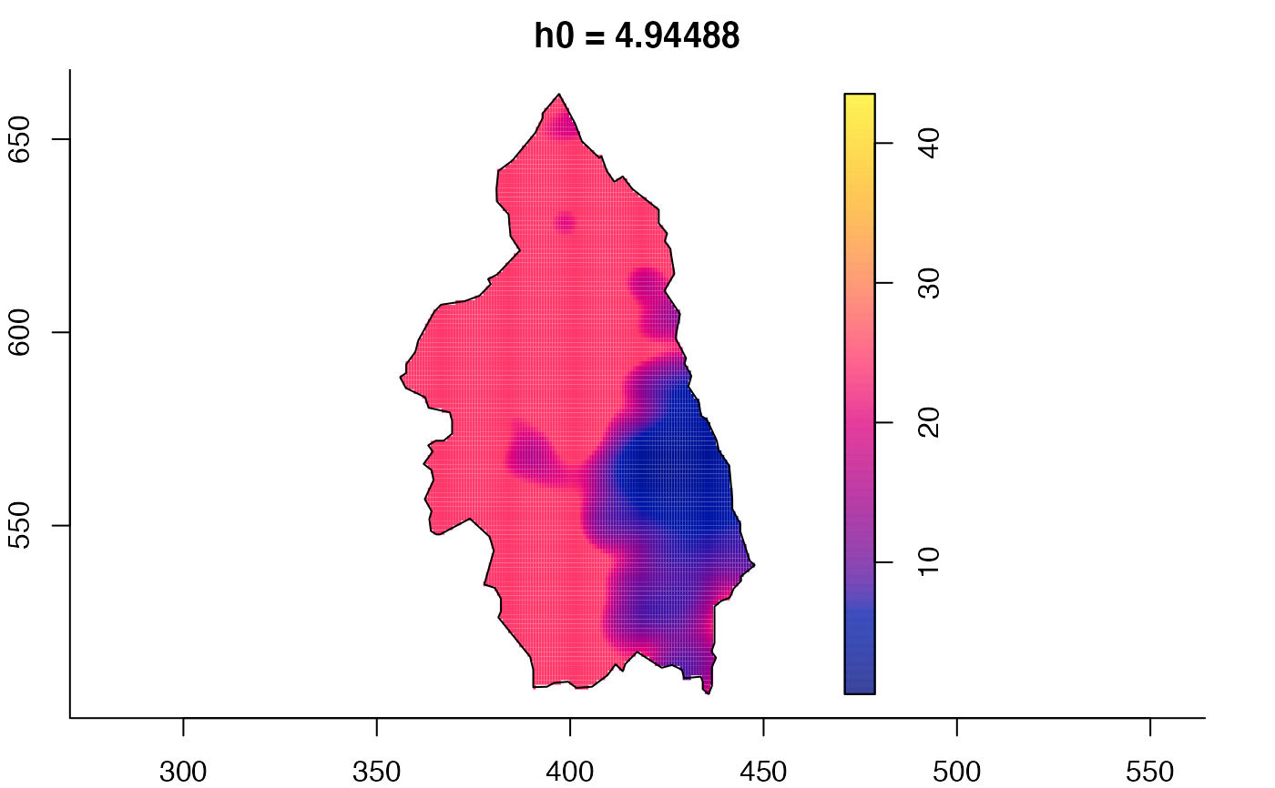
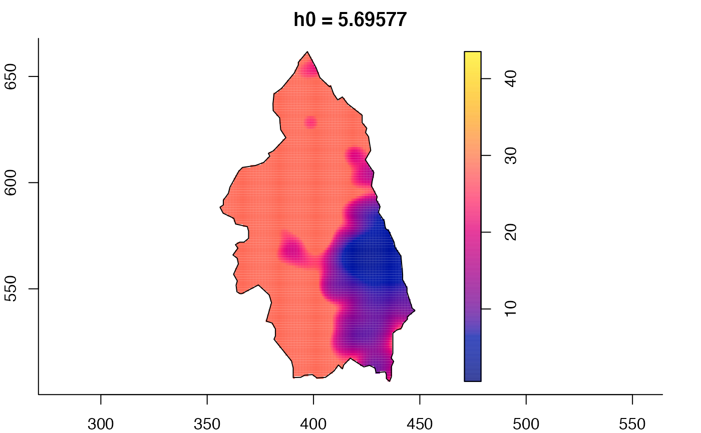
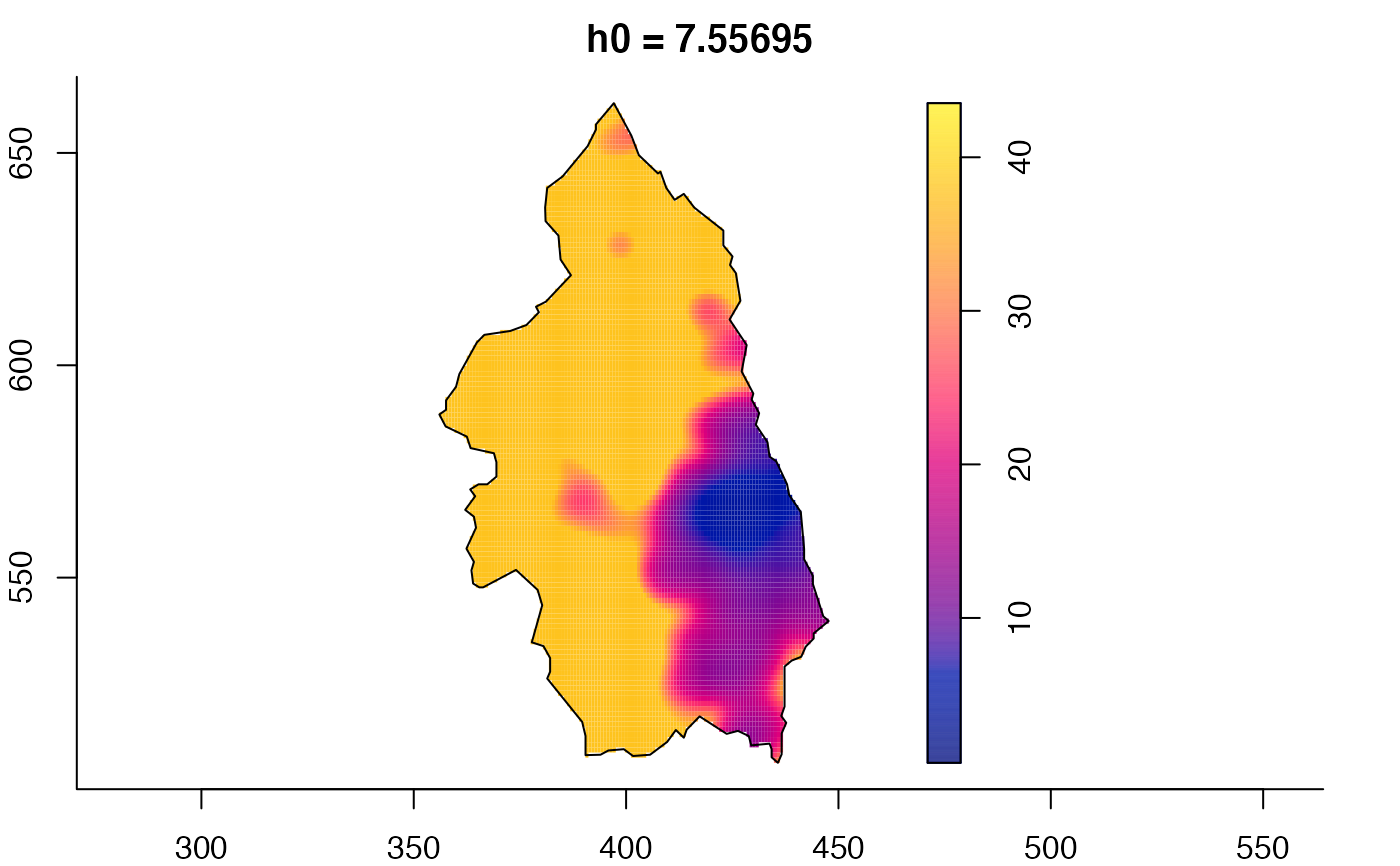
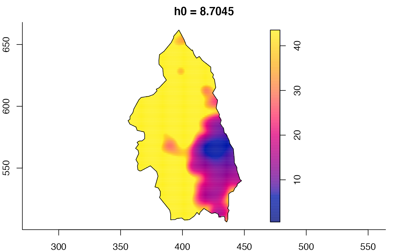
 # 'msden' object
pbcmult <- multiscale.density(split(pbc)$case,h0=4,h0fac=c(0.25,2.5))
#> Initialising...Done.
#> Discretising...Done.
#> Forming kernel...Done.
#> Taking FFT of kernel...Done.
#> Discretising point locations...Done.
#> FFT of point locations...Inverse FFT of smoothed point locations...Done.
#> [ Point convolution: maximum imaginary part= 2.85e-14 ]
#> FFT of window...Inverse FFT of smoothed window...Done.
#> [ Window convolution: maximum imaginary part= 8.78e-15 ]
#> Looking up edge correction weights...
#> 1 2 3 4 5 6 7 8 9 10 11 12 13 14 15 16
plot(pbcmult) # densities
# 'msden' object
pbcmult <- multiscale.density(split(pbc)$case,h0=4,h0fac=c(0.25,2.5))
#> Initialising...Done.
#> Discretising...Done.
#> Forming kernel...Done.
#> Taking FFT of kernel...Done.
#> Discretising point locations...Done.
#> FFT of point locations...Inverse FFT of smoothed point locations...Done.
#> [ Point convolution: maximum imaginary part= 2.85e-14 ]
#> FFT of window...Inverse FFT of smoothed window...Done.
#> [ Window convolution: maximum imaginary part= 8.78e-15 ]
#> Looking up edge correction weights...
#> 1 2 3 4 5 6 7 8 9 10 11 12 13 14 15 16
plot(pbcmult) # densities


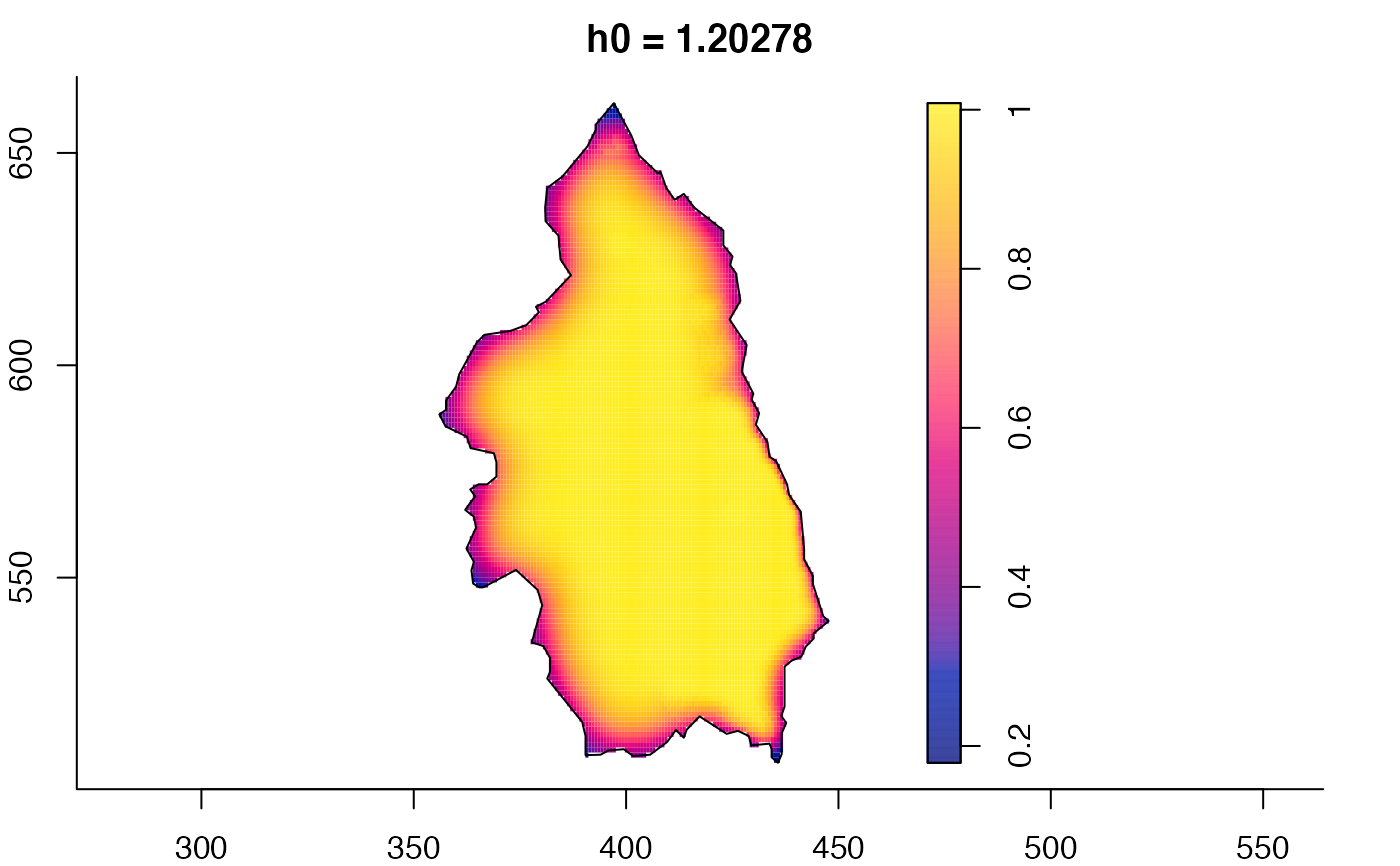
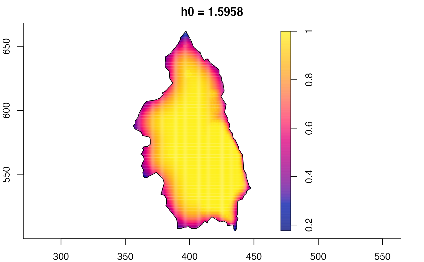
 plot(pbcmult,what="edge") # edge correction surfaces


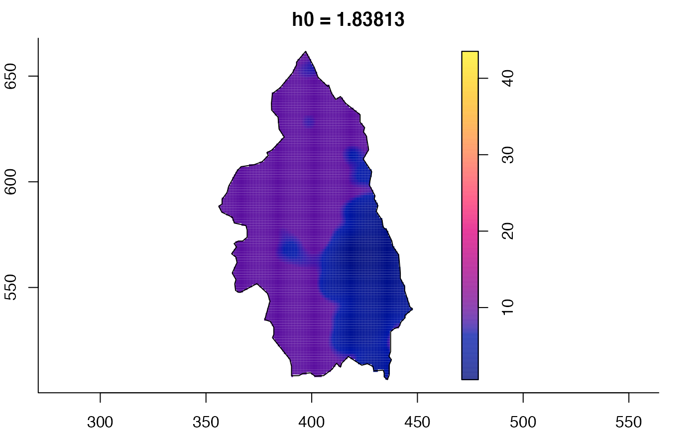
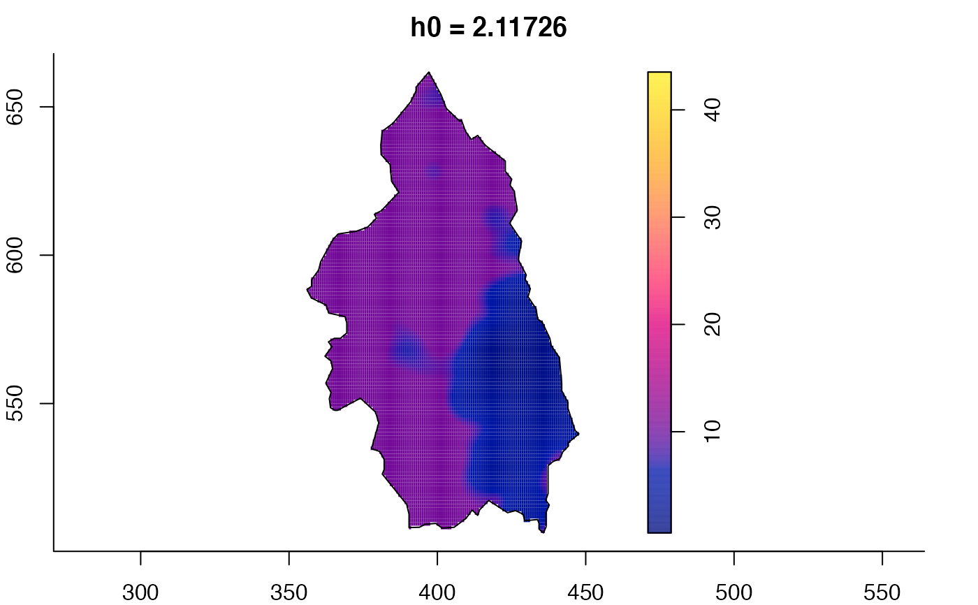
 plot(pbcmult,what="bw") # bandwidth surfaces


 # }
# }