Spatiotemporal kernel density estimation

Provides a fixed-bandwidth kernel estimate of continuous spatiotemporal data.

spattemp.density(pp, h = NULL, tt = NULL, lambda = NULL,
  tlim = NULL, sedge = c("uniform", "none"), tedge = sedge, 
  sres = 128, tres = NULL, verbose = TRUE)

Arguments

pp: An object of class ppp giving the spatial coordinates of the observations to be smoothed. Possibly marked with the time of each event; see argument tt.
h: Fixed bandwidth to smooth the spatial margin. A numeric value > 0. If unsupplied, the oversmoothing bandwidth is used as per OS.
tt: A numeric vector of equal length to the number of points in pp, giving the time corresponding to each spatial observation. If unsupplied, the function attempts to use the values in the marks attribute of the ppp.object in pp.
lambda: Fixed bandwidth to smooth the temporal margin; a numeric value > 0. If unsupplied, the function internally computes the Sheather-Jones bandwith using bw.SJ (Sheather & Jones, 1991).
tlim: A numeric vector of length 2 giving the limits of the temporal domain over which to smooth. If supplied, all times in tt must fall within this interval (equality with limits allowed). If unsupplied, the function simply uses the range of the observed temporal values.
sedge: Character string dictating spatial edge correction. "uniform" (default) corrects based on evaluation grid coordinate. Setting sedge="none" requests no edge correction.
tedge: As sedge, for temporal edge correction.
sres: Numeric value > 0. Resolution of the [sres $\times$ sres] evaluation grid in the spatial margin.
tres: Numeric value > 0. Resolution of the evaluation points in the temporal margin as defined by the tlim interval. If unsupplied, the density is evaluated at integer values between tlim[1] and tlim[2].
verbose: Logical value indicating whether to print a function progress bar to the console during evaluation.

Details

This function produces a fixed-bandwidth kernel estimate of a single spatiotemporal density, with isotropic smoothing in the spatial margin, as per Fernando & Hazelton (2014). Estimates may be edge-corrected for an irregular spatial study window and for the bounds on the temporal margin as per tlim; this edge-correction is performed in precisely the same way as the "uniform" option in bivariate.density.

Specifically, for $n$ trivariate points in space-time (pp, tt, tlim), we have $$\hat{f}(x,t)=n^{-1}\sum_{i=1}^{n}h^{-2}\lambda^{-1}K((x-x_i)/h)L((t-t_i)/\lambda)/(q(x)q(t)),$$ where $x\in W\subset R^2$ and $t\in T\subset R$; $K$ and $L$ are the 2D and 1D Gaussian kernels controlled by fixed bandwidths $h$ (h) and $\lambda$ (lambda) respectively; and $q(x)=\int_W h^{-2}K((u-x)/h)du$ and $q(t)=\int_T \lambda^{-1}L((w-t)/\lambda)dw$ are optional edge-correction factors (sedge and tedge).

The above equation provides the joint or unconditional density at a given space-time location $(x,t)$. In addition to this, the function also yields the conditional density at each grid time, defined as $$\hat{f}(x|t)=\hat{f}(x,t)/\hat{f}(t),$$ where $\hat{f}(t)=n^{-1}\sum_{i=1}^{n}\lambda^{-1}L((t-t_i)/\lambda)/q(t)$ is the univariate kernel estimate of the temporal margin. Normalisation of the two versions $\hat{f}(x,t)$ and $\hat{f}(x|t)$ is the only way they differ. Where in the unconditional setting we have $\int_W\int_T\hat{f}(x,t)dt dx=1$, in the conditional setting we have $\int_W\hat{f}(x|t) dx=1$ for all $t$. See Fernando & Hazelton (2014) for further details and practical reasons as to why we might prefer one over the other in certain situations.

The objects returned by this function (see `Value' below) are necessary for kernel estimation of spatiotemporal relative risk surfaces, which is performed by spattemp.risk.

Value

An object of class "stden". This is effectively a list with the following components:

z: A named (by time-point) list of pixel images corresponding to the joint spatiotemporal density over space at each discretised time.
z.cond: A named (by time-point) list of pixel images corresponding to the conditional spatial density given each discretised time.
h: The scalar bandwidth used for spatial smoothing.
lambda: The scalar bandwidth used for temporal smoothing.
tlim: A numeric vector of length two giving the temporal bound of the density estimate.
spatial.z: A pixel image giving the overall spatial margin as a single 2D density estimate (i.e. ignoring time).
temporal.z: An object of class density giving the overall temporal margin as a single 1D density estimate (i.e. ignoring space).
qs: A pixel image giving the edge-correction surface for the spatial margin. NULL if sedge = "none".
qt: A numeric vector giving the edge-correction weights for the temporal margin. NULL if tedge = "none".
pp: A ppp.object of the spatial data passed to the argument of the same name in the initial function call, with marks of the observation times.
tgrid: A numeric vector giving the discretised time grid at which the spatiotemporal density was evaluated (matches the names of z and z.cond).

References

Duong, T. (2007), ks: Kernel Density Estimation and Kernel Discriminant Analysis for Multivariate Data in R, Journal of Statistical Software, 21(7), 1-16.

Fernando, W.T.P.S. and Hazelton, M.L. (2014), Generalizing the spatial relative risk function, Spatial and Spatio-temporal Epidemiology, 8, 1-10.

Kelsall, J.E. and Diggle, P.J. (1995), Kernel estimation of relative risk, Bernoulli, 1, 3-16.

Sheather, S. J. and Jones, M. C. (1991), A reliable data-based bandwidth selection method for kernel density estimation. Journal of the Royal Statistical Society Series B, 53, 683-690.

Silverman, B.W. (1986), Density Estimation for Statistics and Data Analysis, Chapman & Hall, New York.

Author

T.M. Davies

Examples

data(burk)
burkcas <- burk$cases

burkden1 <- spattemp.density(burkcas,tres=128)
#> Calculating trivariate smooth...
#> Done.
#> Edge-correcting...
#> Done.
#> Conditioning on time...
#> Done.
summary(burkden1)
#> Spatiotemporal Kernel Density Estimate
#> 
#> Bandwidths
#>   h = 11.2439 (spatial)
#>   lambda = 459.5736 (temporal)
#> 
#> No. of observations
#>   188 
#> 
#> Spatial bound
#>   Type: polygonal
#>   2D enclosure: [246.4, 341] x [237.6, 419.4]
#> 
#> Temporal bound
#>   [413, 5775]
#> 
#> Evaluation
#>   128 x 128 x 128 trivariate lattice
#>   Density range: [6.845224e-12, 1.188266e-07]

# \donttest{
hlam <- LIK.spattemp(burkcas,tlim=c(400,5900),verbose=FALSE)
burkden2 <- spattemp.density(burkcas,h=hlam[1],lambda=hlam[2],tlim=c(400,5900),tres=256)
#> Calculating trivariate smooth...
#> Done.
#> Edge-correcting...
#> Done.
#> Conditioning on time...
#> Done.
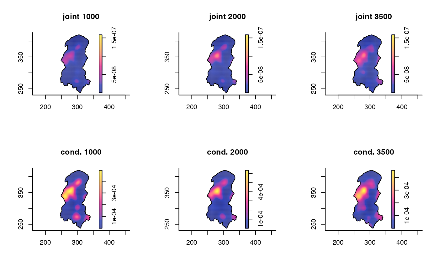
tims <- c(1000,2000,3500)
par(mfcol=c(2,3))
for(i in tims){ 
  plot(burkden2,i,override.par=FALSE,fix.range=TRUE,main=paste("joint",i))
  plot(burkden2,i,"conditional",override.par=FALSE,main=paste("cond.",i))
}

# }