Spatial relative risk/density ratio

Estimates a relative risk function based on the ratio of two 2D kernel density estimates.

risk(
  f,
  g = NULL,
  log = TRUE,
  h0 = NULL,
  hp = h0,
  adapt = FALSE,
  shrink = FALSE,
  shrink.args = list(rescale = TRUE, type = c("lasso", "Bithell"), lambda = NA),
  tolerate = FALSE,
  doplot = FALSE,
  pilot.symmetry = c("none", "f", "g", "pooled"),
  epsilon = 0,
  verbose = TRUE,
  ...
)

Arguments

f

Either a pre-calculated object of class bivden representing the `case' (numerator) density estimate, or an object of class ppp giving the observed case data. Alternatively, if f is ppp object with dichotomous factor-valued marks, the function treats the first level as the case data, and the second as the control data, obviating the need to supply g.

g

As for f, for the `control' (denominator) density; this object must be of the same class as f. Ignored if, as stated above, f contains both case and control observations.

log

Logical value indicating whether to return the (natural) log-transformed relative risk function as recommended by Kelsall and Diggle (1995a). Defaults to TRUE, with the alternative being the raw density ratio.

h0

A single positive numeric value or a vector of length 2 giving the global bandwidth(s) to be used for case/control density estimates; defaulting to a common oversmoothing bandwidth computed via OS on the pooled data using nstar = "geometric" if unsupplied. Ignored if f and g are already bivden objects.

hp

A single numeric value or a vector of length 2 giving the pilot bandwidth(s) to be used for fixed-bandwidth estimation of the pilot densities for adaptive risk surfaces. Ignored if adapt = FALSE or if f and g are already bivden objects.

adapt

A logical value indicating whether to employ adaptive smoothing for internally estimating the densities. Ignored if f and g are already bivden objects.

shrink

A logical value indicating whether to compute the shrinkage estimator of Hazelton (2023). This is only possible for adapt=FALSE.

shrink.args

A named list of optional arguments controlling the shrinkage estimator. Possible entries are rescale (a logical value indicating whether to integrate to one with respect to the control distribution over the window); type (a character string stipulating the shrinkage methodology to be used, either the default "lasso" or the alternative "Bithell"); and lambda (a non-negative numeric value determining the degree of shrinkage towards uniform relative risk---when set to its default NA, it is selected via cross-validation).

tolerate

A logical value indicating whether to internally calculate a corresponding asymptotic p-value surface (for tolerance contours) for the estimated relative risk function. See `Details'.

doplot

Logical. If TRUE, an image plot of the estimated relative risk function is produced using various visual presets. If additionally tolerate was TRUE, asymptotic tolerance contours are automatically added to the plot at a significance level of 0.05 for elevated risk (for more flexible options for calculating and plotting tolerance contours, see tolerance and tol.contour).

pilot.symmetry

A character string used to control the type of symmetry, if any, to use for the bandwidth factors when computing an adaptive relative risk surface. See `Details'. Ignored if adapt = FALSE.

epsilon

A single non-negative numeric value used for optional scaling to produce additive constant to each density in the raw ratio (see `Details'). A zero value requests no additive constant (default).

verbose

Logical value indicating whether to print function progress during execution.

...

Additional arguments passed to any internal calls of bivariate.density for estimation of the requisite densities. Ignored if f and g are already bivden objects.

Value

An object of class "rrs". This is a named list with the following components:

rr

A pixel image of the estimated risk surface.

f

An object of class bivden used as the numerator or `case' density estimate.

g

An object of class bivden used as the denominator or `control' density estimate.

P

Only included if tolerate = TRUE. A pixel image of the p-value surface for tolerance contours; NULL otherwise.

Details

The relative risk function is defined here as the ratio of the `case' density to the `control' (Bithell, 1990; 1991). Using kernel density estimation to model these densities (Diggle, 1985), we obtain a workable estimate thereof. This function defines the risk function r in the following fashion:

r = (fd + epsilon*max(gd))/(gd + epsilon*max(gd)),

where fd and gd denote the case and control density estimates respectively. Note the (optional) additive constants defined by epsilon times the maximum of each of the densities in the numerator and denominator respectively (see Bowman and Azzalini, 1997). A more recent shrinkage estimator developed by Hazelton (2023) is also implemented.

The log-risk function rho, given by rho = log[r], is argued to be preferable in practice as it imparts a sense of symmetry in the way the case and control densities are treated (Kelsall and Diggle, 1995a;b). The option of log-transforming the returned risk function is therefore selected by default.

When computing adaptive relative risk functions, the user has the option of obtaining a so-called symmetric estimate (Davies et al. 2016) via pilot.symmetry. This amounts to choosing the same pilot density for both case and control densities. By choosing "none" (default), the result uses the case and control data separately for the fixed-bandwidth pilots, providing the original asymmetric density-ratio of Davies and Hazelton (2010). By selecting either of "f", "g", or "pooled", the pilot density is calculated based on the case, control, or pooled case/control data respectively (using hp[1] as the fixed bandwidth). Davies et al. (2016) noted some beneficial practical behaviour of the symmetric adaptive surface over the asymmetric.

If the user selects tolerate = TRUE, the function internally computes asymptotic tolerance contours as per Hazelton and Davies (2009) and Davies and Hazelton (2010). When adapt = FALSE, the reference density estimate (argument ref.density in tolerance) is taken to be the estimated control density. The returned pixel image of p-values (see `Value') is interpreted as an upper-tailed test i.e. smaller p-values represent greater evidence in favour of significantly increased risk. For greater control over calculation of tolerance contours, use tolerance.

References

Bithell, J.F. (1990), An application of density estimation to geographical epidemiology, Statistics in Medicine, 9, 691-701.

Bithell, J.F. (1991), Estimation of relative risk functions, Statistics in Medicine, 10, 1745-1751.

Bowman, A.W. and Azzalini A. (1997), Applied Smoothing Techniques for Data Analysis: The Kernel Approach with S-Plus Illustrations, Oxford University Press Inc., New York.

Davies, T.M. and Hazelton, M.L. (2010), Adaptive kernel estimation of spatial relative risk, Statistics in Medicine, 29(23) 2423-2437.

Davies, T.M., Jones, K. and Hazelton, M.L. (2016), Symmetric adaptive smoothing regimens for estimation of the spatial relative risk function, Computational Statistics & Data Analysis, 101, 12-28.

Diggle, P.J. (1985), A kernel method for smoothing point process data, Journal of the Royal Statistical Society Series C, 34(2), 138-147.

Hazelton, M.L. (2023), Shrinkage estimators of the spatial relative risk function, Submitted for publication.

Hazelton, M.L. and Davies, T.M. (2009), Inference based on kernel estimates of the relative risk function in geographical epidemiology, Biometrical Journal, 51(1), 98-109.

Kelsall, J.E. and Diggle, P.J. (1995a), Kernel estimation of relative risk, Bernoulli, 1, 3-16.

Kelsall, J.E. and Diggle, P.J. (1995b), Non-parametric estimation of spatial variation in relative risk, Statistics in Medicine, 14, 2335-2342.

Author

T.M. Davies

Examples

data(pbc)
pbccas <- split(pbc)$case
pbccon <- split(pbc)$control
h0 <- OS(pbc,nstar="geometric")

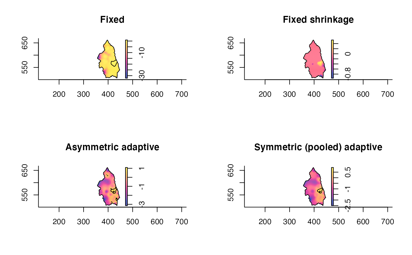
# Fixed (with tolerance contours)
pbcrr1 <- risk(pbccas,pbccon,h0=h0,tolerate=TRUE)
#> Estimating case and control densities...
#> Done.
#> Calculating tolerance contours...
#> Done.

# Fixed shrinkage
pbcrr2 <- risk(pbccas,pbccon,h0=h0,shrink=TRUE,shrink.args=list(lambda=4))
#> Estimating case and control densities...
#> Done.

# Asymmetric adaptive
pbcrr3 <- risk(pbccas,pbccon,h0=h0,adapt=TRUE,hp=c(OS(pbccas)/2,OS(pbccon)/2),
               tolerate=TRUE,davies.baddeley=0.05)
#> Estimating case density...
#> Done.
#> Estimating control density...
#> Done.
#> Calculating tolerance contours...
#> Done.

# Symmetric (pooled) adaptive
pbcrr4 <- risk(pbccas,pbccon,h0=h0,adapt=TRUE,tolerate=TRUE,hp=OS(pbc)/2,
               pilot.symmetry="pooled",davies.baddeley=0.05)
#> Estimating case density...
#> Done.
#> Estimating control density...
#> Done.
#> Calculating tolerance contours...
#> Done.

# Symmetric (case) adaptive; from two existing 'bivden' objects
f <- bivariate.density(pbccas,h0=h0,hp=2,adapt=TRUE,pilot.density=pbccas,
                       edge="diggle",davies.baddeley=0.05,verbose=FALSE) 
g <- bivariate.density(pbccon,h0=h0,hp=2,adapt=TRUE,pilot.density=pbccas,
                       edge="diggle",davies.baddeley=0.05,verbose=FALSE)
pbcrr5 <- risk(f,g,tolerate=TRUE,verbose=FALSE)

par(mfrow=c(2,2))
plot(pbcrr1,override.par=FALSE,main="Fixed")
plot(pbcrr2,override.par=FALSE,main="Fixed shrinkage")
plot(pbcrr3,override.par=FALSE,main="Asymmetric adaptive")
plot(pbcrr4,override.par=FALSE,main="Symmetric (pooled) adaptive")