Multi-scale adaptive kernel density/intensity estimation
Source:R/multiscale.density.R
multiscale.density.RdComputes adaptive kernel estimates of spatial density/intensity using a 3D FFT for multiple global bandwidth scales.
Arguments
- pp
An object of class
pppgiving the observed 2D data set to be smoothed.- h0
Reference global bandwidth for adaptive smoothing; numeric value > 0. Multiscale estimates will be computed by rescaling this value as per
h0fac.- hp
Pilot bandwidth (scalar, numeric > 0) to be used for fixed bandwidth estimation of the pilot density. If
NULL(default), it will take on the value ofh0. Ignored whenpilot.densityis supplied as a pre-defined pixel image.- h0fac
A numeric vector of length 2 stipulating the span of the global bandwidths in the multiscale estimates. Interpreted as a multiplicative factor on
h0. See `Details'.- edge
Character string dictating edge correction.
"uniform"(default) corrects based on evaluation grid coordinate. Settingedge="none"requests no edge correction.- resolution
Numeric value > 0. Resolution of evaluation grid in the spatial domain; the densities/intensities will be returned on a [
resolution\(\times\)resolution] grid.- dimz
Resolution of z- (rescaled bandwidth)-axis in the trivariate convolution. Higher values increase precision of the multiscale estimates at a computational cost. See `Details'.
- gamma.scale
Scalar, numeric value > 0; controls rescaling of the variable bandwidths. Defaults to the geometric mean of the bandwidth factors given the pilot density (as per Silverman, 1986). See the documentation for
bivariate.density.- trim
Numeric value > 0; controls bandwidth truncation for adaptive estimation. See the documentation for
bivariate.density.- intensity
Logical value indicating whether to return an intensity estimate (integrates to the sample size over the study region), or a density estimate (default, integrates to 1).
- pilot.density
An optional pixel image (class
im) giving the pilot density to be used for calculation of the variable bandwidths in adaptive estimation, or appp.objectgiving the data upon which to base a fixed-bandwidth pilot estimate usinghp. See the documentation forbivariate.density.- xy
Optional alternative specification of the spatial evaluation grid; matches the argument of the same tag in
as.mask. If supplied,resolutionis ignored.- taper
Logical value indicating whether to taper off the trivariate kernel outside the range of
h0*h0facin the scale space; see Davies & Baddeley (2018). Keep at the defaultTRUEif you don't know what this means.- verbose
Logical value indicating whether to print function progress.
Value
An object of class "msden". This is very similar to a
bivden object, with lists of pixel
images in the z, him, and q
components (instead of standalone images).
- z
A list of the resulting density/intensity estimates; each member being a pixel image object of class
im. They are placed in increasing order of the discretised values ofh0.- h0
A copy of the reference value of
h0used.- h0range
A vector of length 2 giving the actual range of global bandwidth values available (inclusive).
- hp
A copy of the value of
hpused.- h
A numeric vector of length equal to the number of data points, giving the bandwidth used for the corresponding observation in
ppwith respect to the reference global bandwidthh0.- him
A list of pixel images (class
im), corresponding toz, giving the `hypothetical' Abramson bandwidth at each pixel coordinate conditional upon the observed data and the global bandwidth used.- q
Edge-correction weights; list of pixel
images corresponding tozifedge = "uniform", andNULLifedge = "none".- gamma
The numeric value of
gamma.scaleused in scaling the bandwidths.- geometric
The geometric mean of the untrimmed variable bandwidth factors. This will be identical to
gammaifgamma.scale = "geometric"as per default.- pp
A copy of the
ppp.objectinitially passed to theppargument, containing the data that were smoothed.
Details
Davies & Baddeley (2018) investigated computational aspects of Abramson's (1982) adaptive kernel smoother for spatial (2D) data. This function is the implementation of the 3D convolution via a fast-Fourier transform (FFT) which allows simultaneous calculation of an adaptive kernel estimate at multiple global bandwidth scales.
These `multiple global bandwidth scales' are computed with respect to
rescaling a reference value of the global bandwidth passed to the h0
argument. This rescaling is defined by the range provided to the argument
h0fac. For example, by default, the function will compute the
adaptive kernel estimate for a range of global bandwidths between
0.25*h0 and 1.5*h0. The exact numeric limits are subject to
discretisation, and so the returned valid range of global bandwidths will
differ slightly. The exact resulting range following function execution is
returned as the h0range element of the result, see `Value' below.
The distinct values of global bandwidth used (which define the
aforementioned h0range) and hence the total number of pixel
images returned depend on both the width of the span
h0fac and the discretisation applied to the bandwidth axis through
dimz. Increasing this z-resolution will provide more pixel images and
hence greater numeric precision, but increases computational cost. The
returned pixel images that represent the multiscale
estimates are stored in a named list (see `Value'), whose names reflect the
corresponding distinct global bandwidth. See `Examples' for the easy way to
extract these distinct global bandwidths.
The user can request an interpolated density/intensity estimate for any
global bandwidth value within h0range by using the
multiscale.slice function, which returns an object of class
bivden.
References
Abramson, I. (1982). On bandwidth variation in kernel estimates --- a square root law, Annals of Statistics, 10(4), 1217-1223.
Davies, T.M. and Baddeley A. (2018), Fast computation of spatially adaptive kernel estimates, Statistics and Computing, 28(4), 937-956.
Silverman, B.W. (1986), Density Estimation for Statistics and Data Analysis, Chapman & Hall, New York.
See also
Examples
# \donttest{
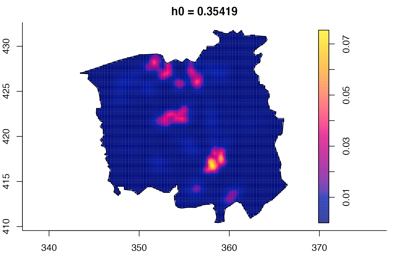
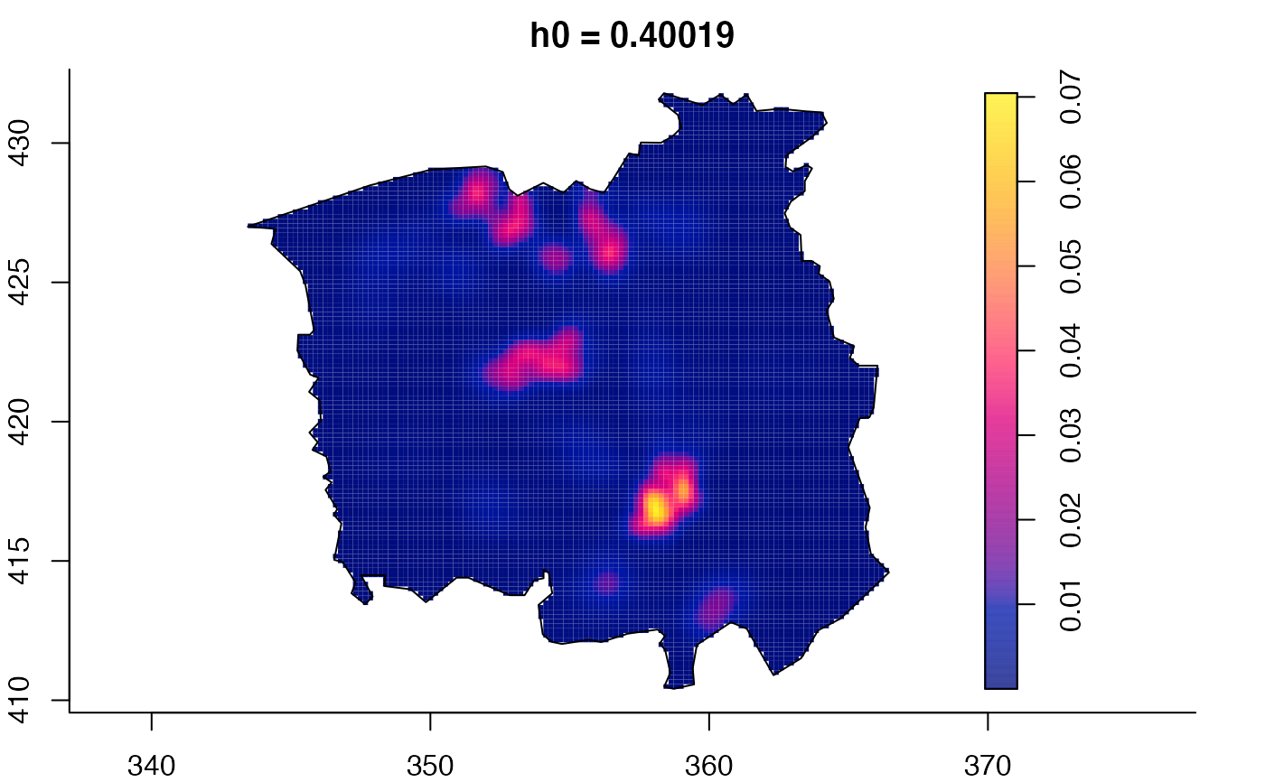
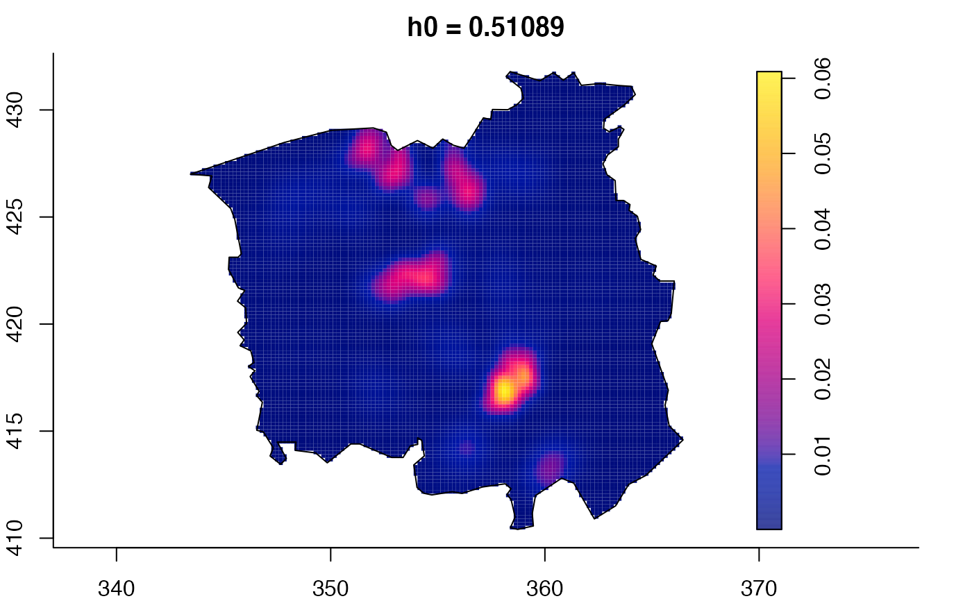
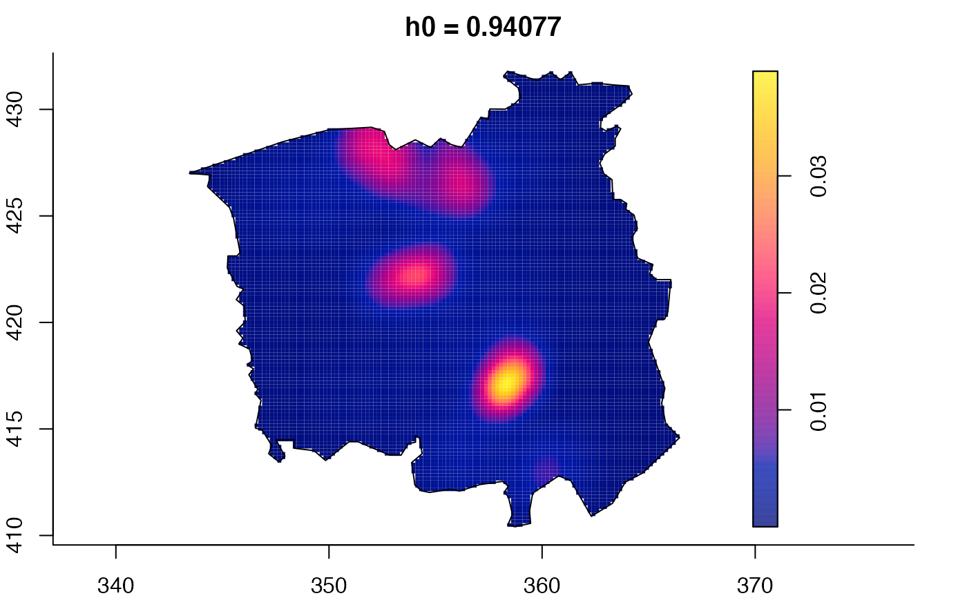
data(chorley) # Chorley-Ribble data (package 'spatstat')
ch.multi <- multiscale.density(chorley,h0=1)
#> Initialising...Done.
#> Discretising...Done.
#> Forming kernel...Done.
#> Taking FFT of kernel...Done.
#> Discretising point locations...Done.
#> FFT of point locations...Inverse FFT of smoothed point locations...Done.
#> [ Point convolution: maximum imaginary part= 2.6e-13 ]
#> FFT of window...Inverse FFT of smoothed window...Done.
#> [ Window convolution: maximum imaginary part= 8.12e-17 ]
#> Looking up edge correction weights...
#> 1 2 3 4 5 6 7 8 9 10 11 12 13 14
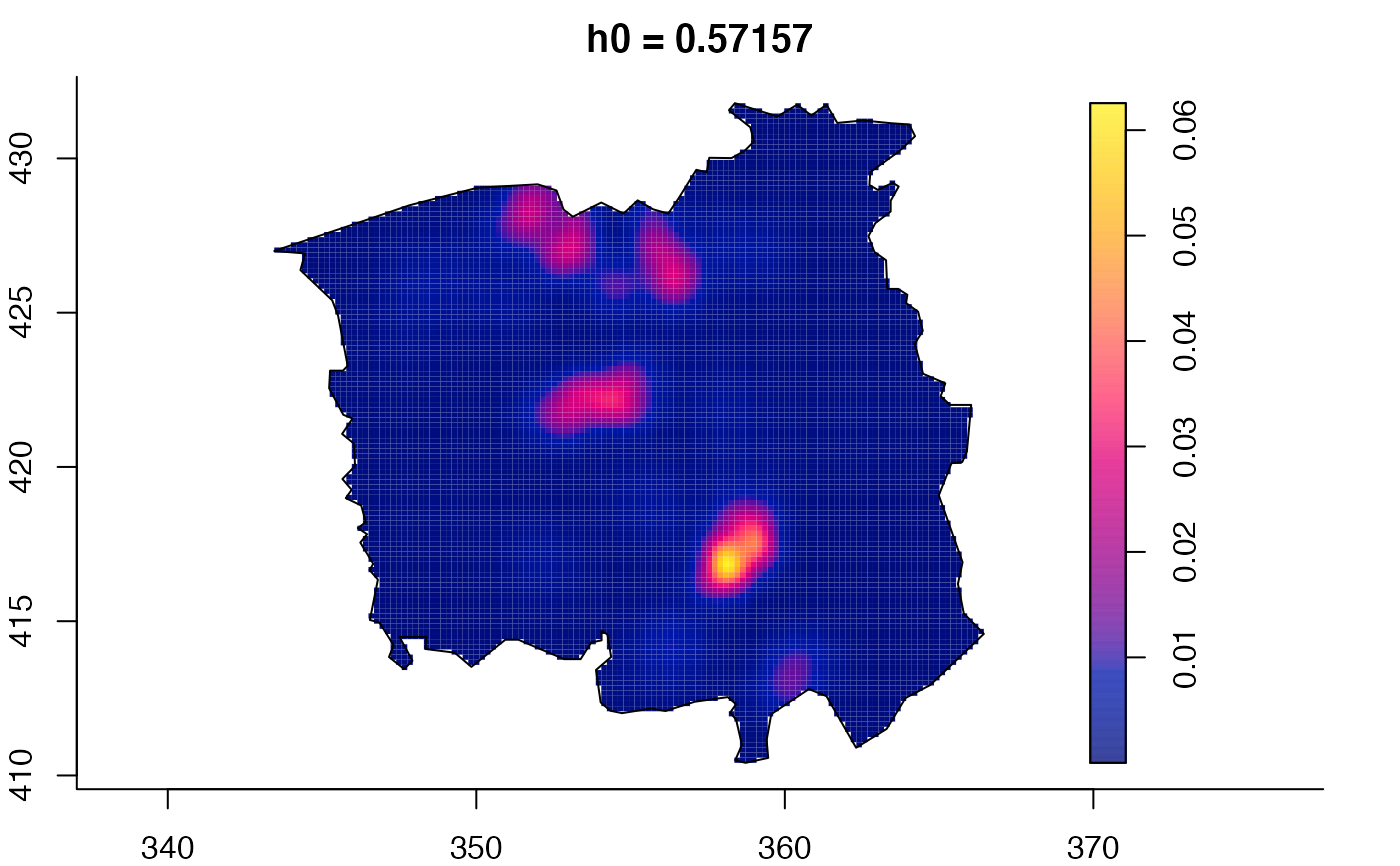
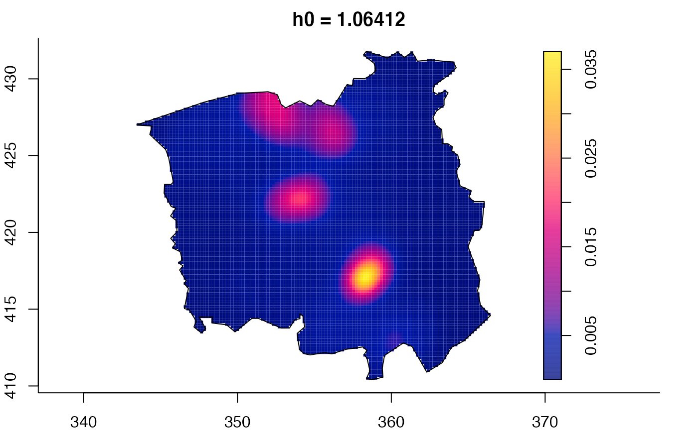
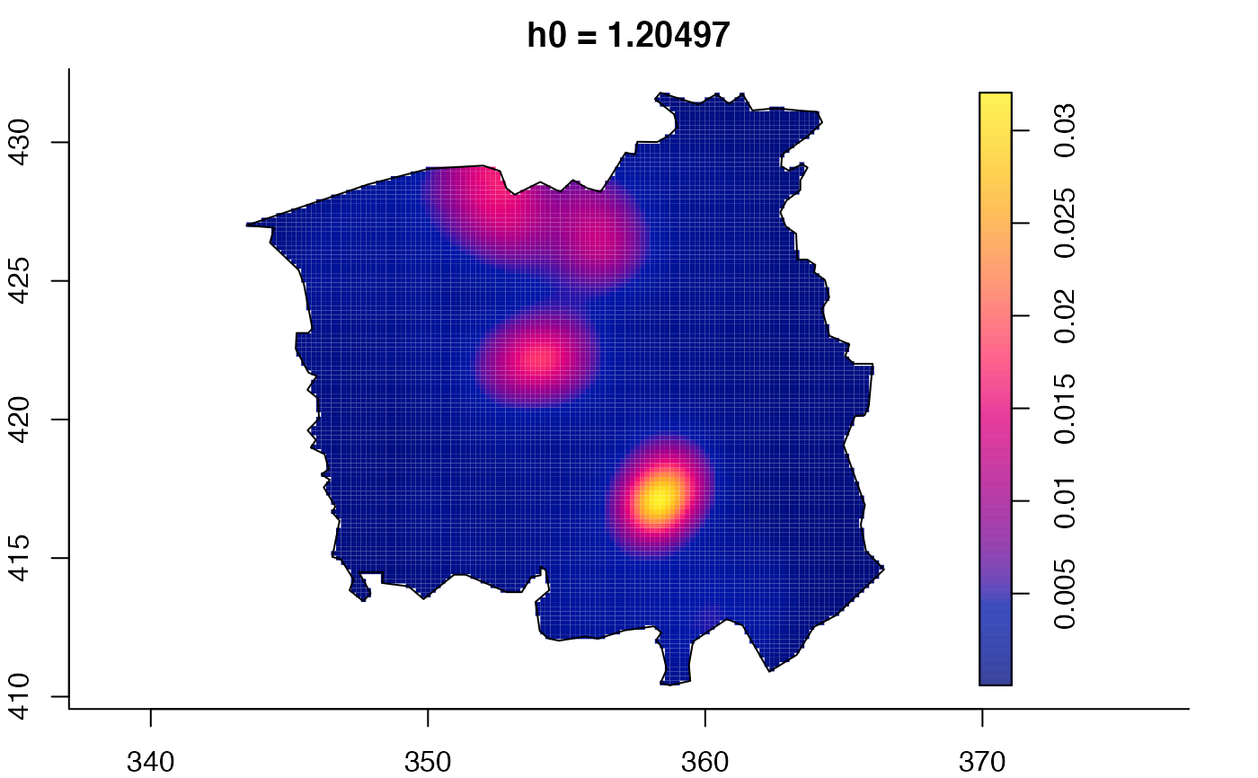
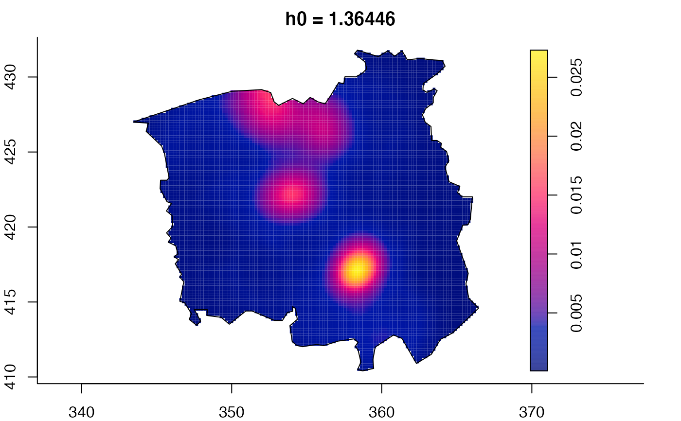
plot(ch.multi)







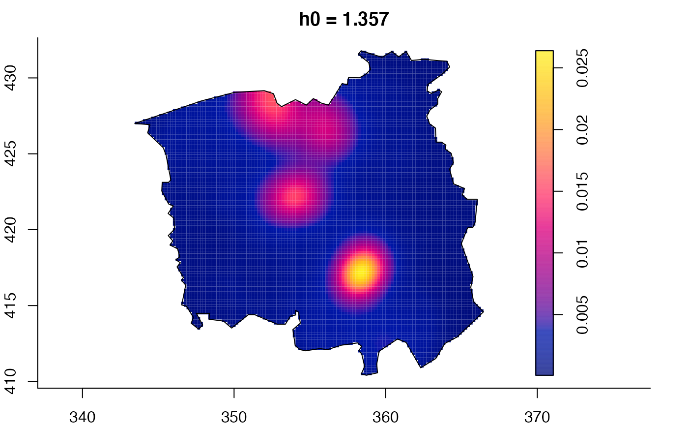 ch.pilot <- bivariate.density(chorley,h0=0.75) # with pre-defined pilot density
ch.multi2 <- multiscale.density(chorley,h0=1,pilot.density=ch.pilot$z)
#> Initialising...Done.
#> Discretising...Done.
#> Forming kernel...Done.
#> Taking FFT of kernel...Done.
#> Discretising point locations...Done.
#> FFT of point locations...Inverse FFT of smoothed point locations...Done.
#> [ Point convolution: maximum imaginary part= 3.35e-13 ]
#> FFT of window...Inverse FFT of smoothed window...Done.
#> [ Window convolution: maximum imaginary part= 9.42e-17 ]
#> Looking up edge correction weights...
#> 1 2 3 4 5 6 7 8 9 10 11 12 13 14
plot(ch.multi2)
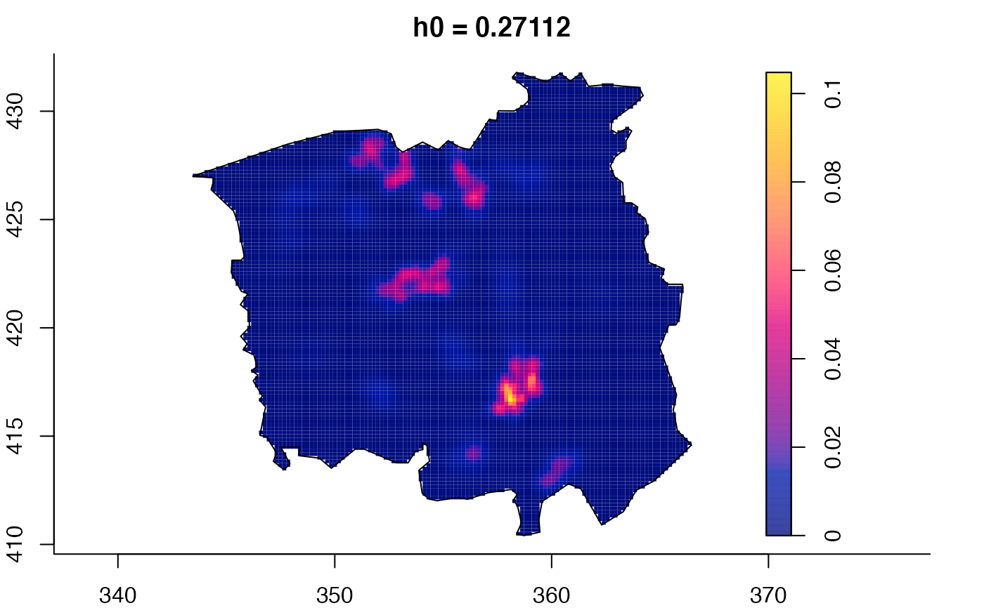

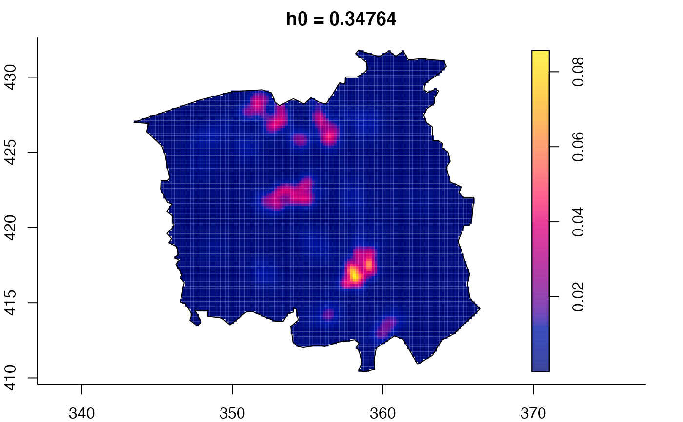

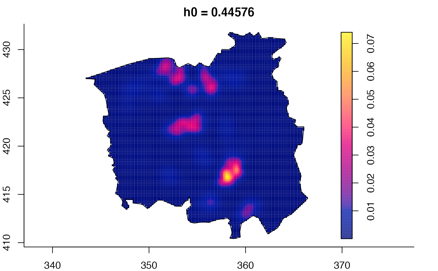



 data(pbc)
# widen h0 scale, increase z-axis resolution
pbc.multi <- multiscale.density(pbc,h0=2,hp=1,h0fac=c(0.25,2.5),dimz=128)
#> Initialising...Done.
#> Discretising...Done.
#> Forming kernel...Done.
#> Taking FFT of kernel...Done.
#> Discretising point locations...Done.
#> FFT of point locations...Inverse FFT of smoothed point locations...Done.
#> [ Point convolution: maximum imaginary part= 1.14e-12 ]
#> FFT of window...Inverse FFT of smoothed window...Done.
#> [ Window convolution: maximum imaginary part= 7.13e-14 ]
#> Looking up edge correction weights...
#> 1 2 3 4 5 6 7 8 9 10 11 12 13 14 15 16 17 18 19 20 21 22 23 24 25 26 27 28 29 30 31
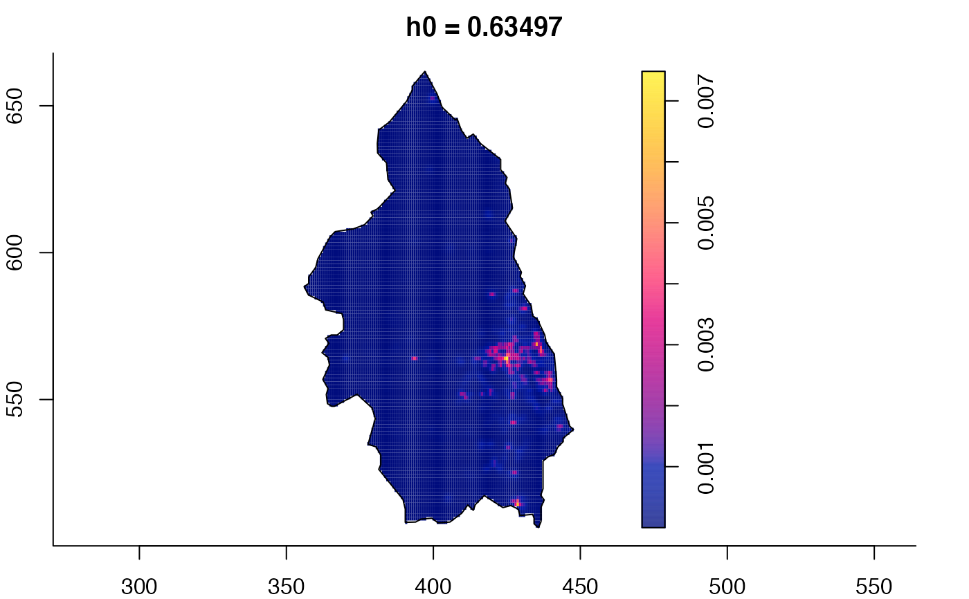
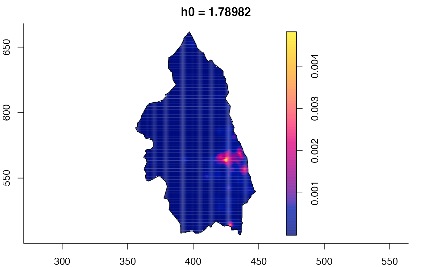
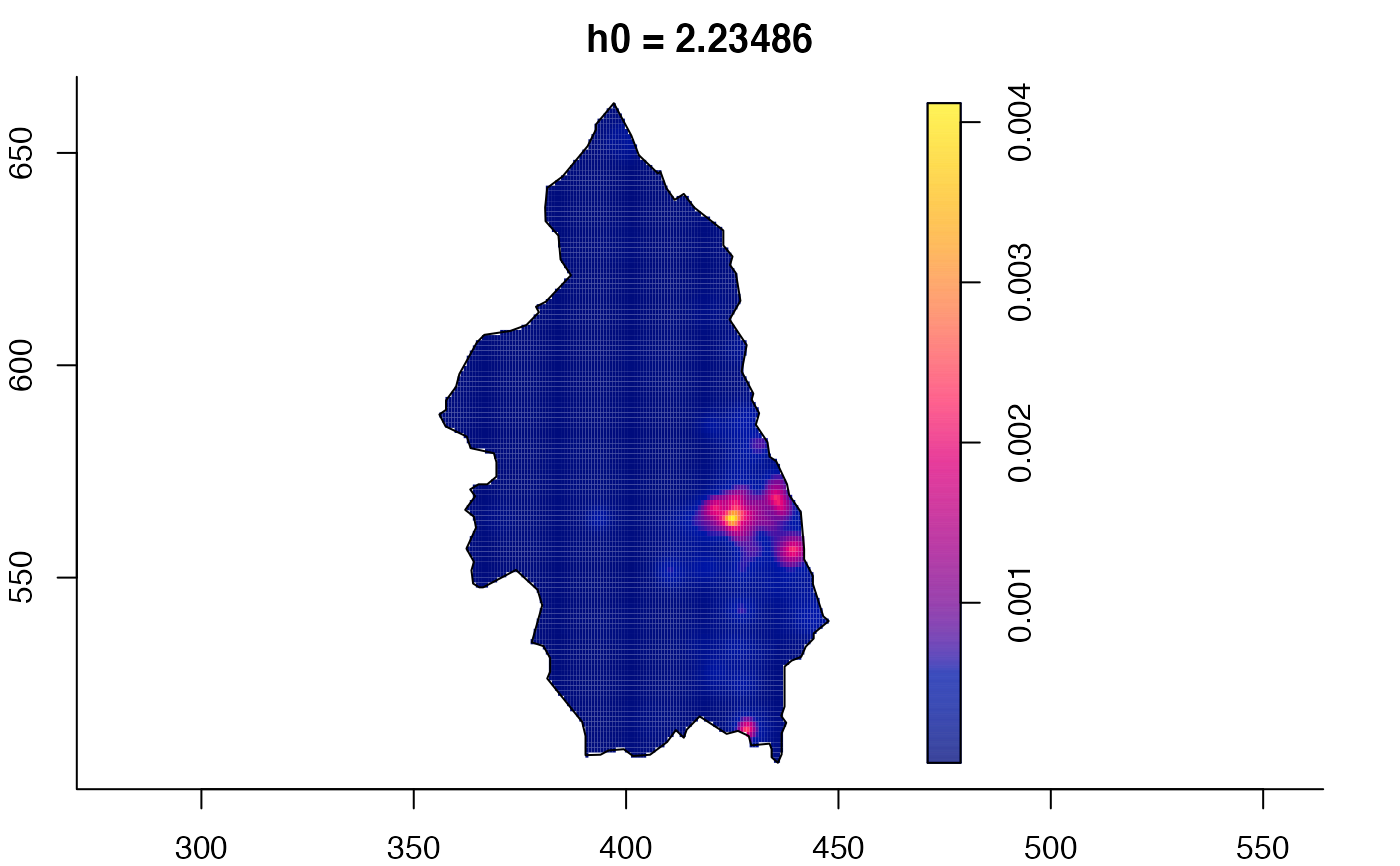
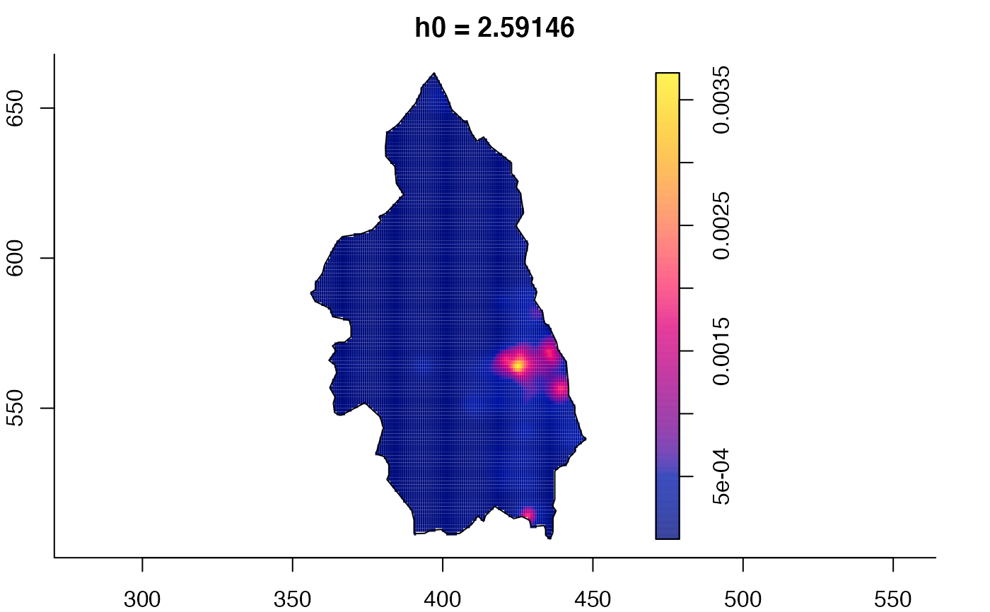
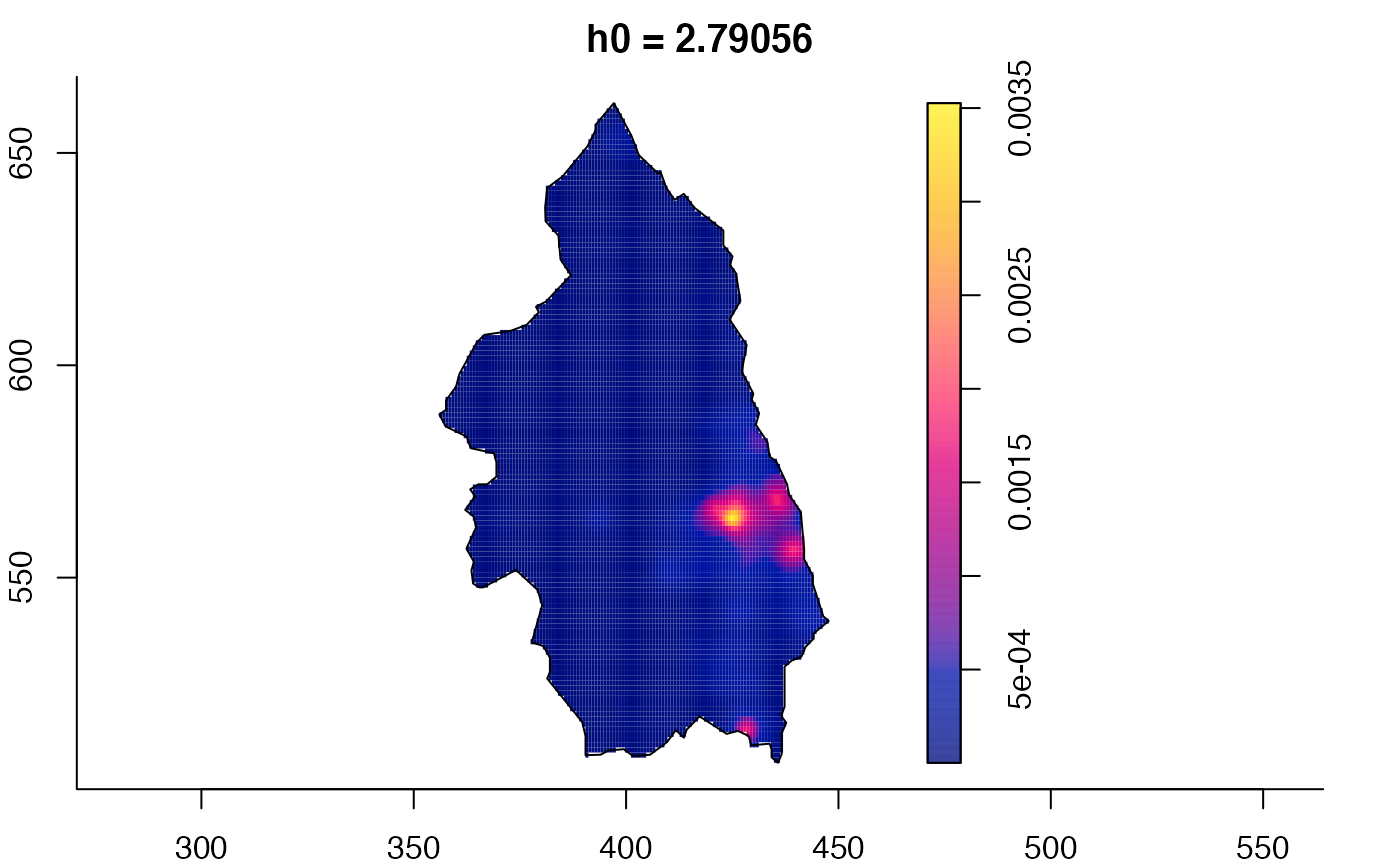
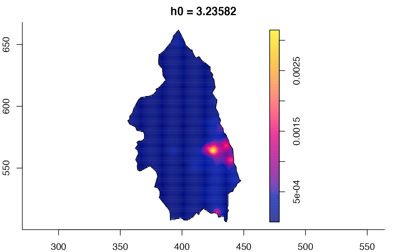
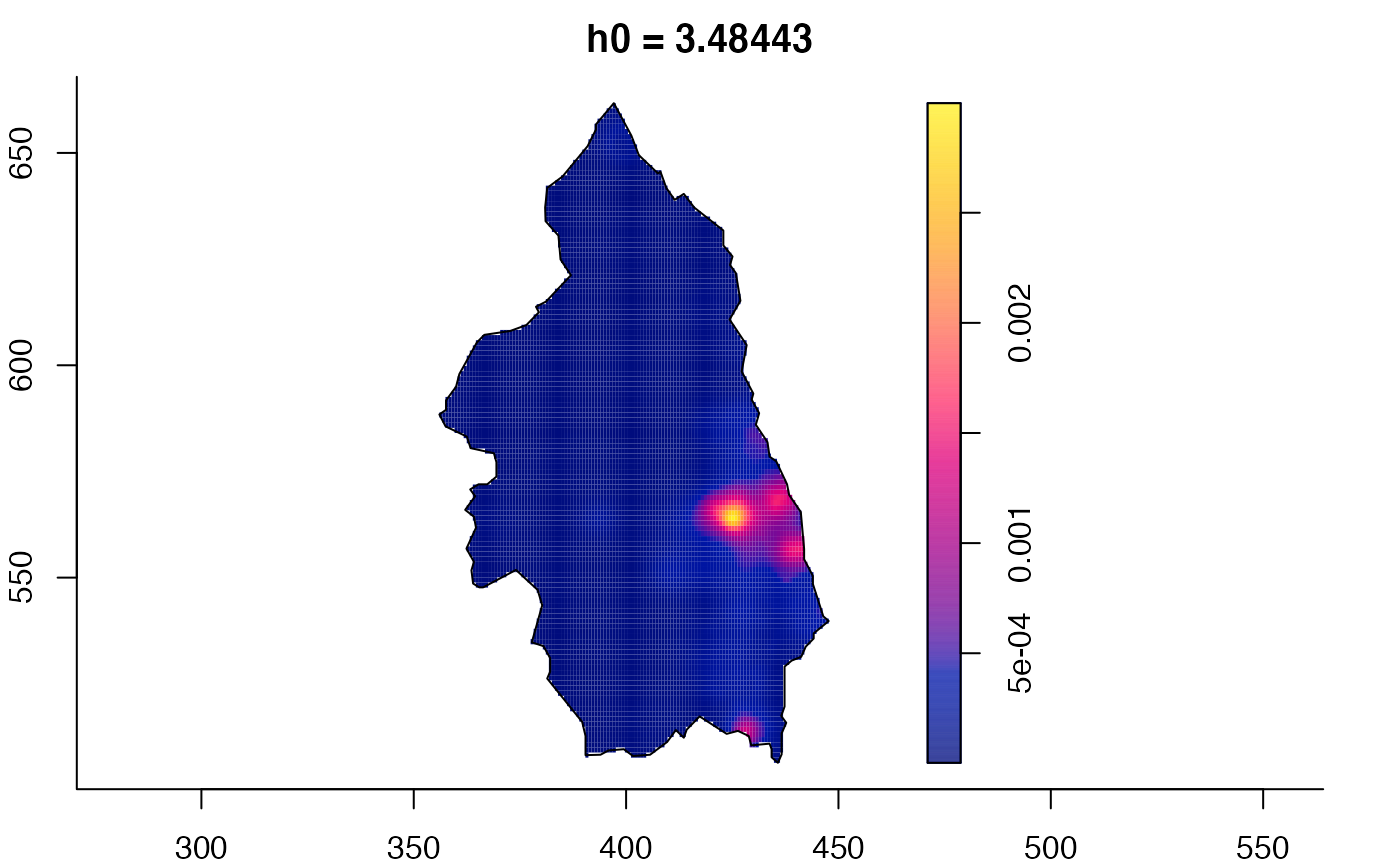
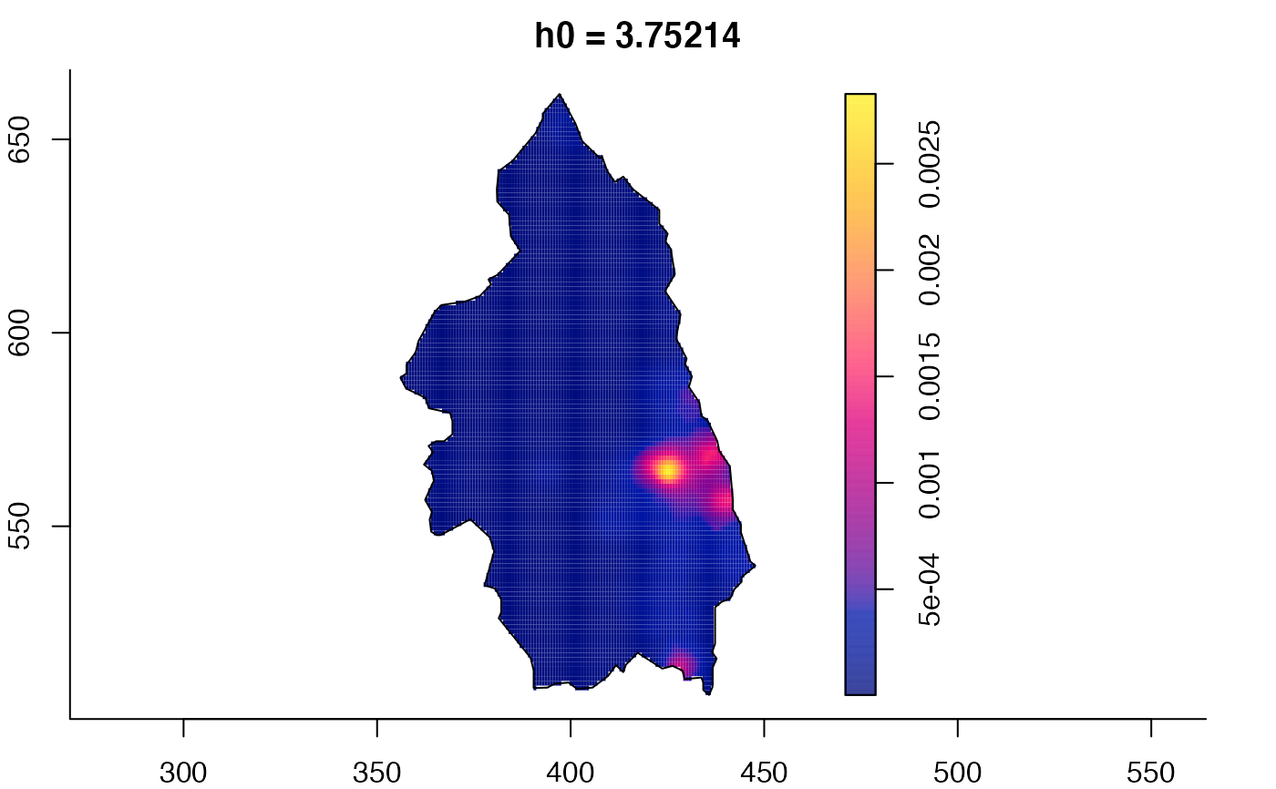
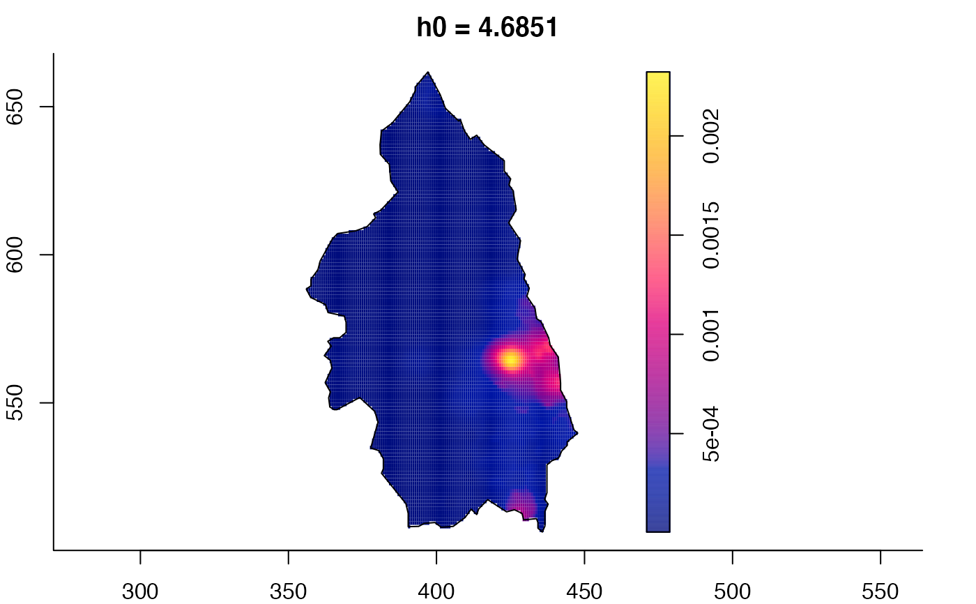
plot(pbc.multi)










 # }
# }