Slicing a multi-scale density/intensity object

Takes slices of a multi-scale density/intensity estimate at desired global bandwidths

multiscale.slice(msob, h0, checkargs = TRUE)

Arguments

msob

An object of class msden giving the multi-scale estimate from which to take slices.

h0

Desired global bandwidth(s); the density/intensity estimate corresponding to which will be returned. A numeric vector. All values must be in the available range provided by msob$h0range; see `Details'.

checkargs

Logical value indicating whether to check validity of msob and h0. Disable only if you know this check will be unnecessary.

Value

If h0 is scalar, an object of class bivden with components corresponding to the requested slice at h0. If h0 is a vector, a list of objects of class bivden.

Details

Davies & Baddeley (2018) demonstrate that once a multi-scale density/intensity estimate has been computed, we may take slices parallel to the spatial domain of the trivariate convolution to return the estimate at any desired global bandwidth. This function is the implementation thereof based on a multi-scale estimate resulting from a call to multiscale.density.

The function returns an error if the requested slices at h0 are not all within the available range of pre-computed global bandwidth scalings as defined by the h0range component of msob.

Because the contents of the msob argument, an object of class msden, are returned based on a discretised set of global bandwidth scalings, the function internally computes the desired surface as a pixel-by-pixel linear interpolation using the two discretised global bandwidth rescalings that bound each requested h0. (Thus, numeric accuracy of the slices is improved with an increase to the dimz argument of the preceding call to multiscale.density at the cost of additional computing time.)

References

Davies, T.M. and Baddeley A. (2018), Fast computation of spatially adaptive kernel estimates, Statistics and Computing, 28(4), 937-956.

See also

multiscale.density, bivariate.density

Author

T.M. Davies

Examples

# \donttest{
data(chorley) # Chorley-Ribble data (package 'spatstat')
ch.multi <- multiscale.density(chorley,h0=1,h0fac=c(0.5,2))
#> Initialising...Done.
#> Discretising...Done.
#> Forming kernel...Done.
#> Taking FFT of kernel...Done.
#> Discretising point locations...Done.
#> FFT of point locations...Inverse FFT of smoothed point locations...Done.
#>   [ Point convolution: maximum imaginary part= 5.09e-14 ]
#> FFT of window...Inverse FFT of smoothed window...Done.
#>   [ Window convolution: maximum imaginary part= 2.67e-17 ]
#> Looking up edge correction weights...
#> 1  2  3  4  5  6  7  8  9  10  11  12  

available.h0(ch.multi)
#> [1] 0.5477611 1.8256134
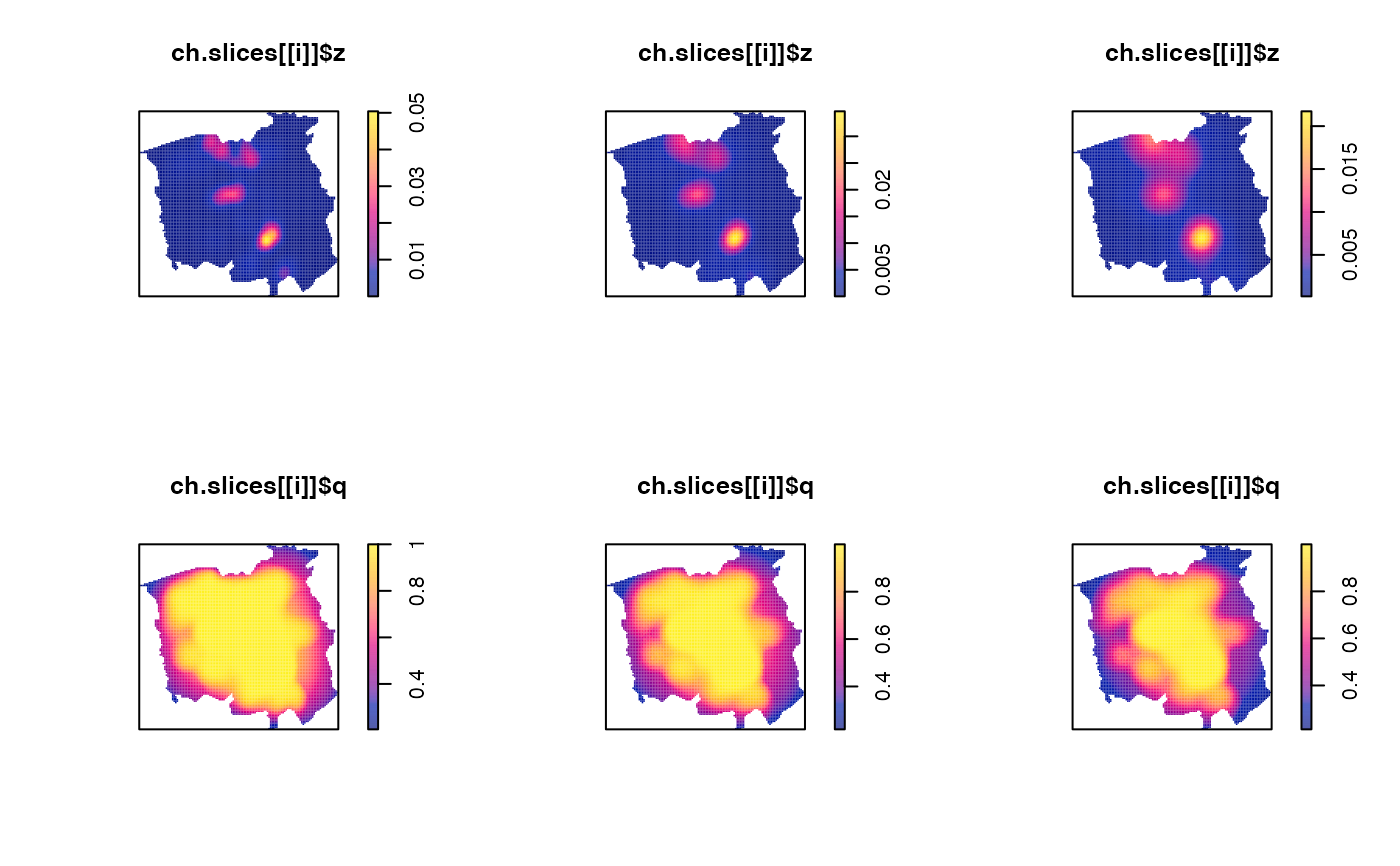
ch.slices <- multiscale.slice(ch.multi,h0=c(0.7,1.1,1.6))

par(mfcol=c(2,3)) # plot each density and edge-correction surface
for(i in 1:3) { plot(ch.slices[[i]]$z); plot(ch.slices[[i]]$q) }

# }